Monte Carlo option pricing with Python: error bars and variance reduction

Published 10 October 2026Updated 15 October 20267 min readOptions pricing:Part 1 Part 2 Part 3 Part 4Part 5Part 6 Part 7 Part 8

Monte Carlo option pricing estimates a discounted payoff expectation under a risk-neutral model. A useful output is a price estimate with a standard error, checked against a known benchmark where one exists.

For a European call under constant-volatility geometric Brownian motion, we can sample the terminal stock price directly. There is no need to discretise a daily path. That gives a clean first project: implement the payoff, verify the stock expectation, compare the estimate with Black–Scholes, then reduce variance without quietly giving one method more work.

This expanded guide uses one synthetic benchmark throughout: spot and strike 100, maturity one year, continuously compounded rate 3%, no dividends, and volatility 20% per square-root year. None of the inputs is a fitted market forecast.

Define the model and the quantity being estimated

Under the risk-neutral measure $\mathbb Q$ ,

S_T=S_0\exp\left((r-q-\tfrac12\sigma^2)T+\sigma\sqrt T Z\right),\qquad Z\sim N(0,1).

For a European call, define the discounted observation

Y=e^{-rT}(S_T-K)^+,

and the price $C=\mathbb E^{\mathbb Q}[Y]$ . Independent copies give the estimator

\widehat C_N=\frac1N\sum_{i=1}^N Y_i.

The $r-q$ drift belongs to the pricing model. Substituting an expected investment return such as 8% changes the distribution and generally gives the wrong no-arbitrage price. More paths would then estimate the wrong expectation more precisely.

The

-\sigma^2/2

term comes from Itô’s lemma. It ensures

\mathbb E^{\mathbb Q}[S_T]=S_0e^{(r-q)T}

. The GBM guide derives the transition, and risk-neutral pricing explains the measure through replication.

Implement plain Monte Carlo

import numpy as np

rng = np.random.default_rng(20261015)
s0, strike, maturity = 100.0, 100.0, 1.0
rate, dividend, sigma = 0.03, 0.0, 0.20
z = rng.standard_normal(200_000)
terminal = s0 * np.exp((rate - dividend - sigma**2 / 2) * maturity
                       + sigma * np.sqrt(maturity) * z)
payoff = np.exp(-rate * maturity) * np.maximum(terminal - strike, 0.0)
price = payoff.mean()
se = payoff.std(ddof=1) / np.sqrt(len(payoff))
print(f"price={price:.6f}, standard error={se:.6f}")
print(f"approximate 95% interval=[{price - 1.96*se:.6f}, {price + 1.96*se:.6f}]")
# price=9.447421, standard error=0.031726
# approximate 95% interval=[9.385238, 9.509604]

The observations are discounted call payoffs, so the standard error has price units. Use ddof=1 for the usual sample variance estimate. The normal interval is an approximate large-sample interval for the model expectation, not a prediction interval for the next realised payoff.

For this European contract, the terminal transition is exact under the model. Sampling error remains, but there is no time-step approximation to refine. If you first generate 252 Euler steps, you add work and numerical error to a problem that does not need either.

Check the analytic benchmark before adding complexity

Under the same assumptions, the Black–Scholes call price is

C=S_0e^{-qT}\Phi(d_1)-Ke^{-rT}\Phi(d_2),

where

d_1=\frac{\log(S_0/K)+(r-q+\sigma^2/2)T}{\sigma\sqrt T},\qquad d_2=d_1-\sigma\sqrt T.

For our inputs, the price is 9.413403. The simulated estimate 9.447421 differs by about 0.0340, or 1.07 estimated standard errors. Its displayed interval includes the benchmark. That is consistent with ordinary finite-sample variation; it is not evidence that the simulation is exact or that every future interval will contain the price.

The downloadable lab implements the normal CDF using the standard-library error function, so the benchmark does not require a separate pricing library. See Black–Scholes explained for the replication argument and assumptions behind the formula.

Also check the simulated stock mean against

100e^{0.03}

. When

q=0

, its discounted mean should be close to 100 within sampling uncertainty. This is a useful unconditional diagnostic. It does not establish the full conditional martingale property.

Interpret convergence correctly

For IID payoffs with finite variance, standard error scales as $N^{-1/2}$ . Four times the draws roughly halves it. A single running estimate can move farther from the benchmark when more draws are added; convergence does not require monotonic improvement along each realised sequence.

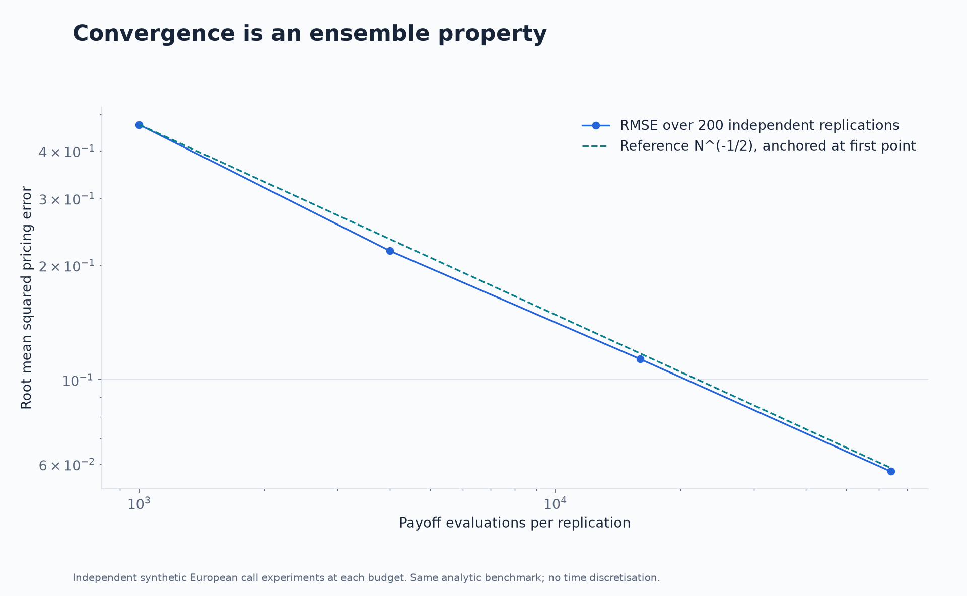
European call pricing root mean squared error declines approximately with the inverse square root of the evaluation budget across independent replications

Each point above uses 200 independent replications at its own budget. We calculate the root mean squared difference from the analytic benchmark. The dashed line is a square-root-rate reference anchored at the first observed point, rather than a fitted claim about all possible sample sizes.

A fixed seed is useful for reproducing an example. Independent replications are useful for studying the estimator’s sampling behaviour. They serve different purposes, and rerunning the identical seed does not provide new evidence about coverage.

For the distinction between sampling error, model uncertainty and grid error, use the general Monte Carlo simulation guide.

Antithetic sampling: the pair is the observation

For each independent Gaussian draw $Z_i$ , evaluate the payoff at both $Z_i$ and $-Z_i$ . Each has the correct marginal distribution. Define

A_i=\frac{Y(Z_i)+Y(-Z_i)}2.

Then $\mathbb E[A_i]=C$ . A monotone call payoff produces negatively related pair outcomes under this model, which reduces the variance of their average relative to two independent observations.

The two payoffs in one pair are dependent. Calculate the standard error from independent pair means:

\widehat{\mathrm{SE}}_{\mathrm{anti}}=\frac{s_A}{\sqrt M},

where $M$ is the number of pairs. Treating all $2M$ payoffs as independent gives an incorrect uncertainty calculation.

At an evaluation budget of 200,000, the fair comparison is 200,000 plain payoffs against 100,000 antithetic pairs. Comparing 200,000 pairs against 200,000 plain payoffs would double the antithetic method’s work before assessing its statistical benefit.

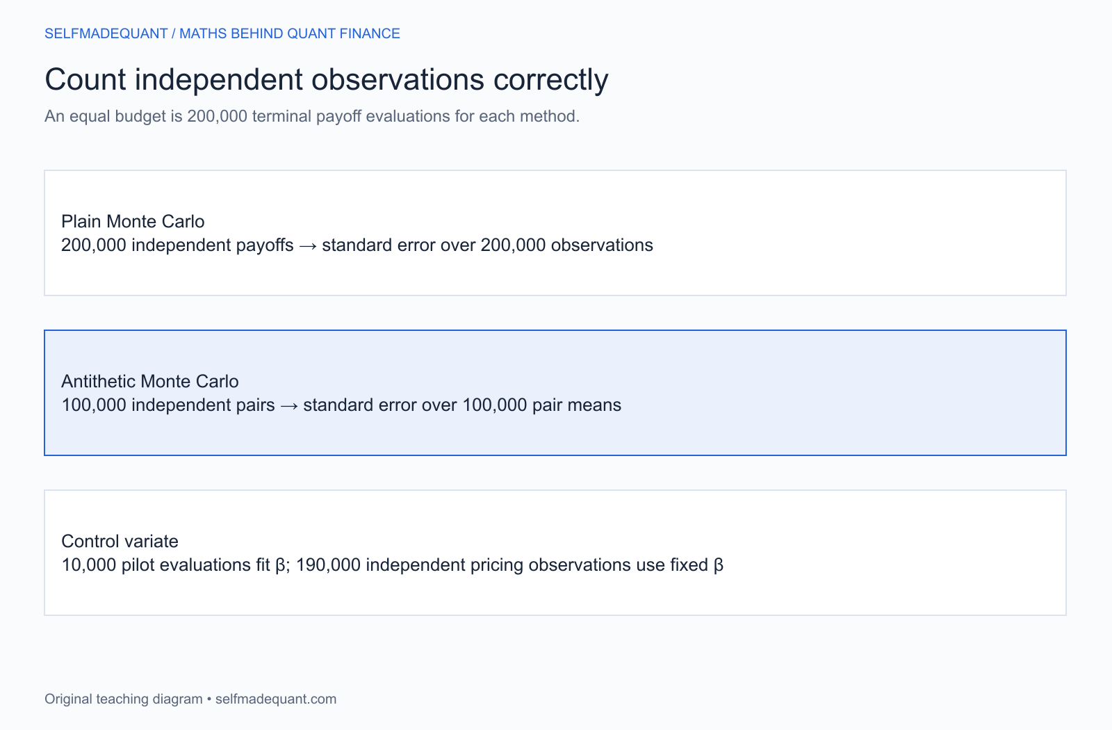
Plain, antithetic and control-variate methods use different independent observation units even when all receive 200000 terminal payoff evaluations

Antithetics do not guarantee a useful reduction for every payoff. A nonmonotone contract can behave differently. Measure the actual estimator variance rather than assuming that a symmetric construction always helps.

Control variates: remove a known-mean component

The discounted stock

X=e^{-rT}S_T

has known expectation $m_X=S_0e^{-qT}$ . Construct

Y^{\mathrm{cv}}=Y-\beta(X-m_X).

For a fixed $\beta$ , the expected option price is unchanged. The variance-minimising coefficient is $\operatorname{Cov}(Y,X)/\operatorname{Var}(X)$ when the control variance is positive.

The financial relationship is straightforward: a call payoff and terminal stock share much of their movement. Subtracting a correlated quantity with known mean can leave a less variable residual.

Our implementation estimates $\beta$ from an independent pilot of 10,000 evaluations, freezes it, and prices on 190,000 new independent observations. The pilot is included in the total 200,000 budget. Conditional on the pilot coefficient, the production estimator is unbiased and its sample standard error describes the production residuals. The reported interval remains a large-sample approximation.

Estimating $\beta$ on the pricing observations themselves complicates the clean fixed-coefficient argument. An independent pilot keeps the reasoning and the implementation easy to inspect.

Results at one equal evaluation budget

Method	Price estimate	Estimated standard error	Independent pricing observations
Plain	9.447421	0.031726	200,000 payoffs
Antithetic	9.417818	0.023481	100,000 pair means
Control variate	9.410266	0.013319	190,000 residuals after a 10,000-draw pilot

Each method uses 200,000 terminal payoff evaluations. All intervals in this run include the analytic price 9.413403. The control coefficient fitted in the pilot is approximately 0.632709.

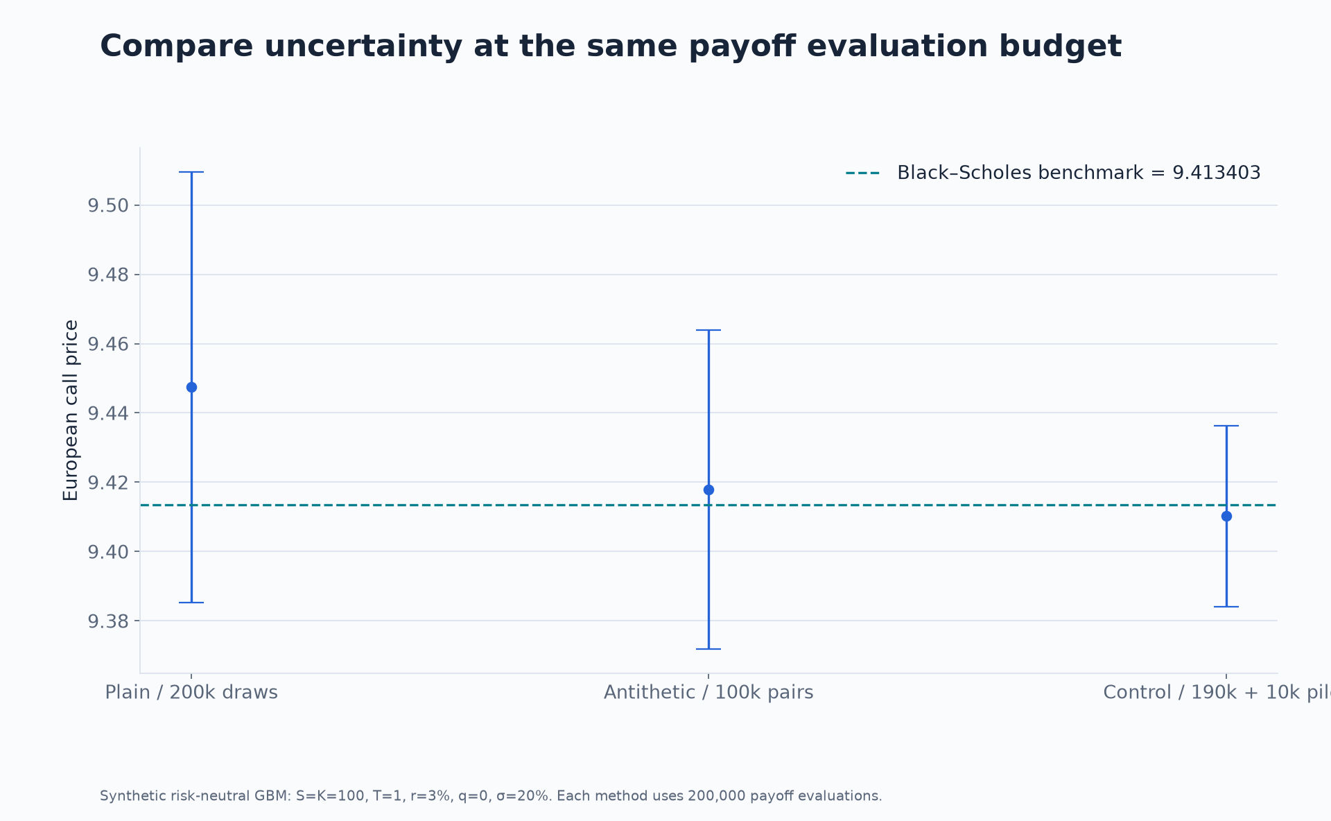
European call estimates with approximate 95 percent intervals show lower reported uncertainty for antithetic and control-variate methods at the same evaluation budget

The comparison is about estimator precision. The control estimate happens to be closest to the benchmark in this run, but closeness in one realisation is not the definition of a better estimator. Compare variance, bias and cost across repeated experiments when evaluating a method.

Equal payoff counts are transparent here, but they do not guarantee equal wall-clock time. Different implementations have different overheads, memory use and opportunities for vectorisation. A performance claim would need timing measurements in a specified environment; this chart makes no such claim.

Path-dependent contracts need a different simulation state

An arithmetic Asian call depends on the average of specified stock observations. A barrier depends on whether a level was crossed. A basket depends on several assets and their joint dynamics. You must simulate the state required by the contract rather than reuse a terminal European payoff unchanged.

Exact GBM transitions at monthly dates price a monthly-observed average when the averaging rule is implemented correctly. They do not automatically price a continuously monitored average or barrier. A continuously monitored barrier can be crossed and recrossed between observation dates. Compatible Brownian-bridge methods can address between-date crossing probabilities under suitable models.

For a general diffusion without an exact transition, a numerical scheme introduces time-discretisation error. Study both path count and time step. More paths reduce sampling variation around the discretised model; they do not remove its bias.

For a basket, specify the covariance model and validate the simulated dependence. For an arithmetic Asian control variate, a related geometric Asian payoff can be useful when its expectation is known under the same observation and model assumptions.

American exercise is a separate decision problem

A terminal payoff simulation does not represent early exercise. An American option requires comparing immediate exercise with conditional continuation at each allowed date. The extra exercise right cannot reduce value relative to the otherwise identical European contract, although it need not add value in every case.

Longstaff–Schwartz estimates continuation values by regression during backward induction. The regression state, exercise grid and policy evaluation all matter. A fitted policy should be valued on independent paths to reduce look-ahead effects from reusing its fitting observations.

The expected value of a particular admissible exercise policy cannot exceed the true optimal value, but a finite-sample policy estimate can fluctuate. That distinction matters when calling something a lower bound.

The new download covers European Monte Carlo estimators, not an American Monte Carlo implementation. The existing option-pricing Python lab and Options Pricing resources remain available for the broader series, including its tree-based American example. Use binomial option pricing to study the exercise recursion first.

Download the code and extend it carefully

The stochastic-calculus resource collection contains a runnable Python lab, the complete estimator functions, recorded outputs and chart files. Run the supplied benchmark before changing the strike, maturity or volatility. Keep the risk-neutral drift, discount convention and dividend treatment consistent across simulation and analytic comparison.

For structured study, use the Options Pricing programme, particularly Monte Carlo option pricing and Longstaff–Schwartz.

This page belongs to the existing Options Pricing series and also completes the maths sequence from martingales through Brownian motion, Itô’s lemma, GBM and risk-neutral valuation. The shared URL keeps this pricing intent in one place.

Sources and further study

MIT’s Analytics of Finance lecture materials offer a computational-finance continuation. Longstaff and Schwartz’s original paper develops regression-based American valuation. The European estimator comparison and all reported figures here were generated from the stated synthetic benchmark.