What does an option price actually mean?

A stock trades at $100. You can buy a contract that lets you purchase it for $100 one year from now. If the stock finishes at $120, the contract pays $20. If it finishes at $80, you walk away.

What should you pay today?

The strike and expiry specify a contract. They do not specify its price. We also need to understand uncertainty, funding, dividends, and which risks trading can remove. Before reaching for Black–Scholes, a tree, or a simulation, make the cash flows precise.

Option pricing starts with replication and no-arbitrage. Risk-neutral valuation writes the resulting price as a discounted expectation; martingales describe the conditional-expectation restriction behind those pricing weights. We will build that connection with a two-state example before using continuous-time models.

Start with the contract

A European call gives its holder the right to buy at strike $K$ at expiry $T$. Its payoff per underlying unit is:

A put pays $(K-S_T)^+$. European describes the exercise rule, not the exchange's location. An American option allows exercise before expiry. A barrier option may cease to exist when a level is hit. An Asian option uses an average. Those details change the valuation problem before we choose a model.

Our teaching contract has $S_0=100$, $K=100$, and $T=1$ year. Rates are continuously compounded. Unless stated otherwise, we use $r=5\%$, continuous dividend yield $q=2\%$, and annual volatility $\sigma=20\%$. Prices are per underlying unit, with no assumed exchange contract multiplier. All numerical examples are synthetic.

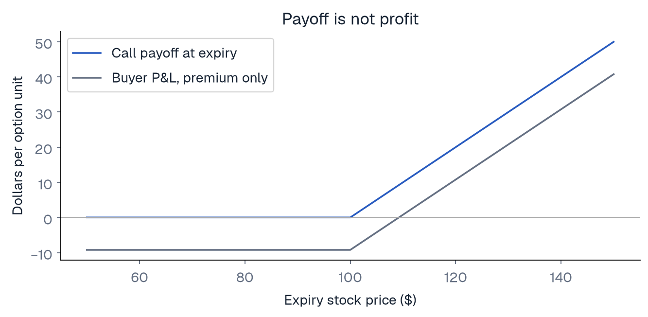
The buyer's expiry profit is not the payoff. Subtract the premium, and include its financing if you measure all cash flows at expiry. A $20 payoff does not tell us whether the buyer made money without knowing the price paid.

Why a forecast is insufficient

Suppose your forecast says the stock has a 60% chance of reaching $120 and a 40% chance of reaching $80. The expected call payoff is $12. Discounting that number at a risk-free rate does not generally produce its no-arbitrage price.

The stock and option are risky. An investor's forecasts and risk preferences matter when valuing unhedgeable claims. But a claim that can be replicated using traded assets has a sharper restriction: two portfolios delivering the same cash flows must have the same price, under the frictionless trading assumptions.

To see this without continuous-time machinery, set dividends to zero and take a one-period bank growth factor of 1.05. Buy $\Delta$ shares and put $B$ dollars in the bank. Replicating the call requires:

Subtract the equations. Then $\Delta=0.5$ and $B=-40/1.05=-38.0952$. The initial cost is $50-38.0952=11.9048$. The negative bank position is borrowing, not a negative option payoff.

If the call trades materially above that amount in this ideal market, selling it and buying the replicating portfolio locks in the difference. If it trades below, reverse the positions. Real funding, shorting restrictions, spreads, and hedge errors complicate execution; they do not change what the ideal calculation demonstrates.

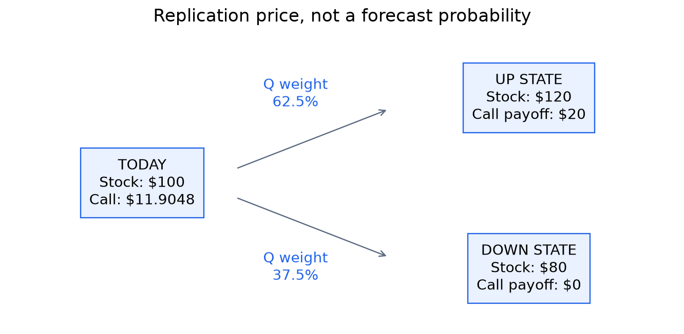
Notice what disappeared: our 60% forecast. Both states are replicated, so that forecast cannot change the replication cost.

Martingales and risk-neutral option pricing

A martingale is an integrable process whose expected future value, conditional on the information available now, equals its current value. For a process $M_t$ under a probability measure $\mathbb Q$:

Here $\mathcal F_t$ represents information available at time $t$. A martingale can move substantially along a realised path. The equality concerns a conditional expectation under a specified measure, not a promise that the next price stays unchanged.

We can write the same price using a probability $p^*$ that makes the discounted stock a martingale:

The call price becomes $0.625\times20/1.05=11.9048$. This is the replication cost written as a discounted expectation. The 62.5% probability is not a prediction about the stock. It is a pricing weight consistent with the stock and bank prices in this model.

Check the stock as well as the option: $(0.625\times120+0.375\times80)/1.05=100$. The expected discounted stock equals today's stock price. Using the original 60% forecast instead gives $104/1.05=99.0476$. That forecast can express an investment view, but it is not the risk-neutral probability for this stock-and-bank model.

For a continuously dividend-paying stock and constant rates, the familiar form is:

The expectation uses the pricing measure $\mathbb Q$. With stochastic rates, discounting generally sits inside the expectation, or we change numeraire and measure carefully. With incomplete markets, no-arbitrage may allow several pricing measures. A particular calibrated model then contains additional choices about unhedgeable risk.

No-arbitrage bounds and put–call parity

For a European call with deterministic $r$ and continuous yield $q$, basic bounds are:

For our inputs the lower bound is approximately $2.90$. It is the difference between prepaid stock and discounted strike, floored at zero. Using $S_0-K$ instead ignores carry and discounting.

European put–call parity is:

At expiry, long call and short put deliver $S_T-K$. Prepaid stock and a borrowing position deliver the same amount. That is why the identity holds. It is not an empirical correlation to estimate. American contracts require different treatment because exercise times can differ.

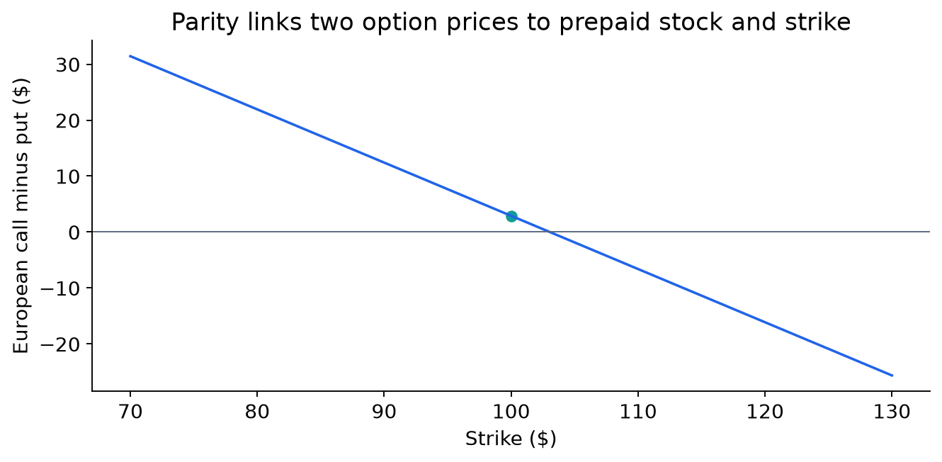
These restrictions are powerful debugging tools. A negative price, a parity failure, or a call that falls when spot increases should trigger investigation before we celebrate numerical precision. Bid and ask data complicate the test: executable arbitrage conditions use the appropriate sides of the market, fees, and funding.

Separate three choices

The payoff tells us what the contract pays. The model tells us how the underlying and other state variables behave under a pricing measure. The solver tells us how we compute the value.

Black–Scholes uses a constant-volatility diffusion and admits a closed-form European vanilla price. A binomial tree approximates a process and discounts backwards. Monte Carlo samples scenarios. Fourier pricing integrates a transform of the distribution. Several solvers can price the same model; a solver can also be used with different models.

This distinction prevents a common comparison error. If a Heston price differs from a Black–Scholes price, the difference may be economic assumptions. If a Black–Scholes Monte Carlo estimate differs slightly from its formula, it may be sampling error. Those are different questions and need different checks.

Try it

Change the bank growth factor in our one-step example from 1.05 to 1.02. Keep terminal stock prices at $120 and $80. The hedge stays at half a share, but borrowing costs change. The price becomes $50-40/1.02=10.7843$. The pricing probability becomes $(102-80)/40=0.55$. Verify that discounting the weighted $20 payoff gives the same result.

Continue learning

Sources