Fourier option pricing: compute the price from a characteristic function

Black–Scholes gives a European call price using normal cumulative probabilities. Monte Carlo estimates the same price by drawing terminal stocks. Fourier pricing reaches it through a different representation of the distribution.

Why bother changing representation?

For some models, the probability density is awkward to write down but the characteristic function is tractable. That includes important stochastic-volatility and jump models. A transform method can exploit what we know analytically rather than simulate every payoff.

The transform is a computational tool. It does not choose the market model, estimate its parameters, or remove model risk.

The risk-neutral characteristic function

Let $X_T=\log S_T$. Its characteristic function under the pricing measure is:

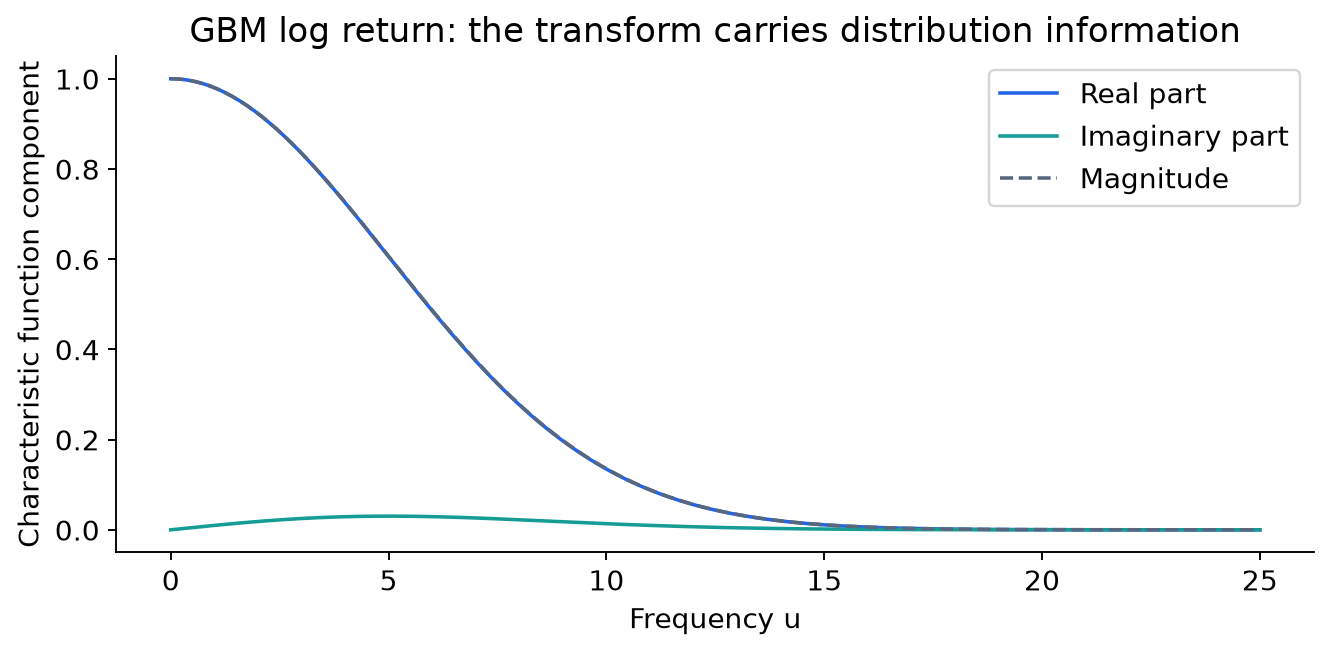
For real $u$, this complex-valued function encodes the terminal distribution. Differentiating at zero can recover moments when they exist; Fourier inversion can recover a density under suitable conditions.

Under our GBM benchmark:

Check two anchors. $\phi_T(0)=1$ because a distribution has total probability one. The analytic continuation at $u=-i$ equals $\mathbb E[S_T]=S_0e^{(r-q)T}$. That second check targets the pricing drift.

Real-valued characteristic functions are not required. Complex arithmetic is part of the method. Throwing away imaginary components before the inversion changes the answer.

Carr–Madan Fourier pricing and damping

Write strike as $K=e^k$ and call value as $C(k)$. A direct Fourier transform in log strike faces an integrability problem: as strike approaches zero, a call's price does not decay to zero.

Carr and Madan multiply the price by $e^{\alpha k}$ for a positive damping parameter $\alpha$. The damped function can be integrable when the relevant moments exist. With constant discounting, its transform is:

The call value follows by inversion:

This is a transform identity under its integrability conditions. The numerical work is now a one-dimensional integral over frequencies.

The shifted argument $v-i(\alpha+1)$ explains why not every positive $\alpha$ is safe in every model. We need a finite moment of order $\alpha+1$. GBM has all positive moments, but other models can have a restricted moment domain. An arbitrary damping parameter can take the characteristic function outside the admissible strip.

Price the same call before changing models

The lab implements that integral using GBM's characteristic function, with $\alpha=1.5$ and an integration upper limit of 150. It returns $9.22700550815404$ for the benchmark call. The direct BSM formula returns $9.227005508154036$.

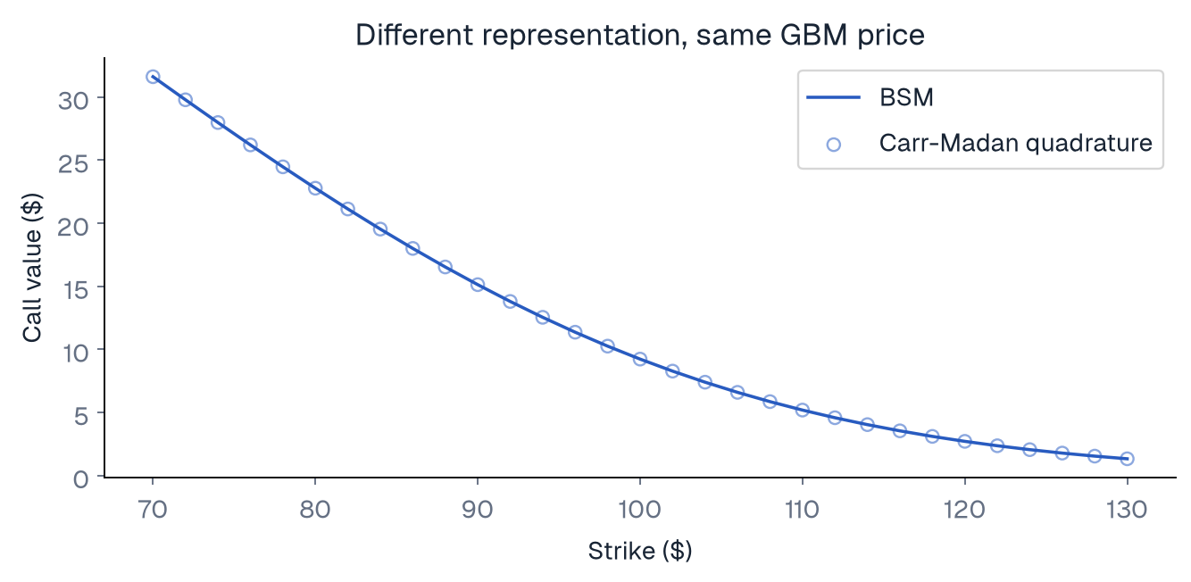
This order matters. If we begin with a complicated Heston implementation and disagree with another system, we do not know whether the fault is the characteristic function, complex branches, transform convention, or integration grid. Recovering BSM first removes several uncertainties.

The quadrature routine's reported error estimate applies to its finite numerical integral. It does not include the omitted tail beyond the chosen upper limit, floating-point issues in the model's characteristic function, or model misspecification. The lab separately varies damping and checks multiple strikes. A production implementation needs broader regimes, including short expiries and extreme moneyness.

Quadrature and FFT are related, but different

For a few strikes, direct quadrature is straightforward: run the integral at each desired $k$. For a large evenly spaced log-strike grid, the fast Fourier transform can compute many related sums efficiently.

Let frequency spacing be $\eta$, with $N$ points. The corresponding log-strike spacing is:

That coupling is important. Frequency truncation, frequency resolution, strike resolution, and the strike range cannot be adjusted independently by wishful thinking. Increasing $N$ at fixed $\eta$ refines the strike grid and expands the maximum frequency; changing $\eta$ also changes the strike range.

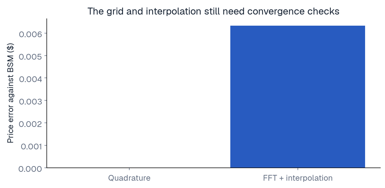
The lab includes a transparent FFT implementation with trapezoidal weights. With $N=4096$ and $\eta=0.05$, interpolating to strike $100$ gives $9.2333$. Its error is about $0.0063$, noticeably larger than the quadrature error. The desired strike falls between grid nodes, so interpolation contributes.

That result is useful precisely because it is imperfect. “Uses FFT” is not a certificate of high accuracy. Grid choices and interpolation need convergence checks. If only a handful of strikes matter, adaptive quadrature may be easier to control than a whole FFT grid.

Heston and Merton jump-diffusion characteristic functions

For lognormal jumps with $\log J\sim N(m_J,s_J^2)$, one representation is:

where $k_J=e^{m_J+s_J^2/2}-1$. The jump compensation makes the expected stock carry consistent with $r-q$. A missing compensator can look like a calibration error while actually being an invalid drift.

For Heston, complex square roots and logarithms need a consistent representation across the integration grid. Branch discontinuities can corrupt an otherwise valid formula. Use established stable formulations, limiting cases, and independent benchmarks. We explain the model here, but our downloadable lab deliberately validates the GBM transform rather than claiming a tested Heston calibration engine.

What this method does not solve by itself

A terminal characteristic function is particularly convenient for European payoffs. It does not automatically encode early exercise or path history. There are transform extensions for other contracts, but they require more machinery and assumptions.

Fourier pricing also depends on the quality of its calibrated inputs. A fast calculation of a misspecified distribution remains a misspecified price. Its strength is computational: it can turn a difficult distributional problem into an integral or grid sum with clear numerical checks.

Try it

Change damping from 1.5 to 0.5, 1.0, and 2.0 in the GBM lab. Increase the integration limit to 200. The result should remain stable to the stated tolerance. Then change the FFT grid and record errors against BSM. Keep model inputs fixed; this is a solver experiment.

Continue learning

Sources