Martingales explained: fair games, conditional expectation and finance

Published 15 October 20266 min readThe maths behind quant finance:Part 1Part 2 Part 3 Part 4 Part 5 Part 6

A martingale is a model of a fair game relative to a specified flow of information: your conditional expected future value equals your current value. It can rise, fall and have substantial risk. The condition concerns what you can predict from what you already know.

That distinction matters in finance. A discounted asset can be a martingale under a pricing probability measure without being a good forecast of realised returns. A betting strategy called “the martingale system” can double after losses without satisfying the conditions needed to turn an optional-stopping argument into a profit claim.

This article develops the idea from a two-step game, then connects it to Brownian motion, discounting and option pricing. You need basic probability and expectations; the beginner maths guide maps the prerequisites.

A six-stage reading roadmap connects martingales, Brownian motion, Itô’s lemma, GBM and risk-neutral pricing to Monte Carlo estimation

What is a martingale?

Let $M_t$ be a random value at time $t$ , and let $\mathcal F_t$ represent all information available by that time. A process is a martingale under probability measure $\mathbb P$ when it is adapted to that information, has $\mathbb E^{\mathbb P}[|M_t|]<\infty$ , and satisfies

\mathbb E^{\mathbb P}[M_t\mid\mathcal F_s]=M_s,\qquad s\leq t.

“Adapted” means that the value at time $s$ is known using information available at $s$ . The integrability condition ensures the expectations are well defined. The final equality is the fair-game condition.

Read the equation as: after using everything currently observed, the average of possible future values is the value you have now. In a discrete-time game, checking the one-step condition at every date is enough to establish the multi-step condition by repeated conditioning.

The information specification belongs in the definition. A price process that looks unpredictable from yesterday’s prices could become predictable if the observer also knew tomorrow’s earnings announcement. It is incomplete to call a process a martingale without saying under which probability law and information flow.

The martingale condition compares a conditional future average with the current value; a constant unconditional mean alone is insufficient

A fair random walk, worked through

Start with $M_0=0$ . At each step, add $+1$ or $-1$ , independently with equal probability. After observing the first step, suppose you have $M_1=1$ . The next value is either 2 or 0, each with probability one half:

\mathbb E[M_2\mid M_1=1]=\tfrac12(2)+\tfrac12(0)=1.

If the first step was a loss, the next value is either 0 or $-2$ :

\mathbb E[M_2\mid M_1=-1]=\tfrac12(0)+\tfrac12(-2)=-1.

Both branches satisfy the same conditional equality. That is stronger than saying the overall average at date 2 is zero.

This walk is risky. After two steps, its possible values are $-2,0,2$ with probabilities $1/4,1/2,1/4$ . Its variance is 2 even though its expected gain is zero. Fairness does not mean that the next result is close to the current value, and it does not mean every realised participant breaks even.

You can verify the branches without simulation:

from itertools import product

paths = list(product((-1, 1), repeat=2))
for first in (-1, 1):
    future = [a + b for a, b in paths if a == first]
    print(first, sum(future) / len(future))
# -1 -1.0
# 1 1.0

Independence is sufficient for this construction, but it is not part of the general martingale definition. Increments can have state-dependent variance and remain conditionally mean zero. A process can therefore be a martingale while its volatility is predictable.

Why a constant mean is not enough

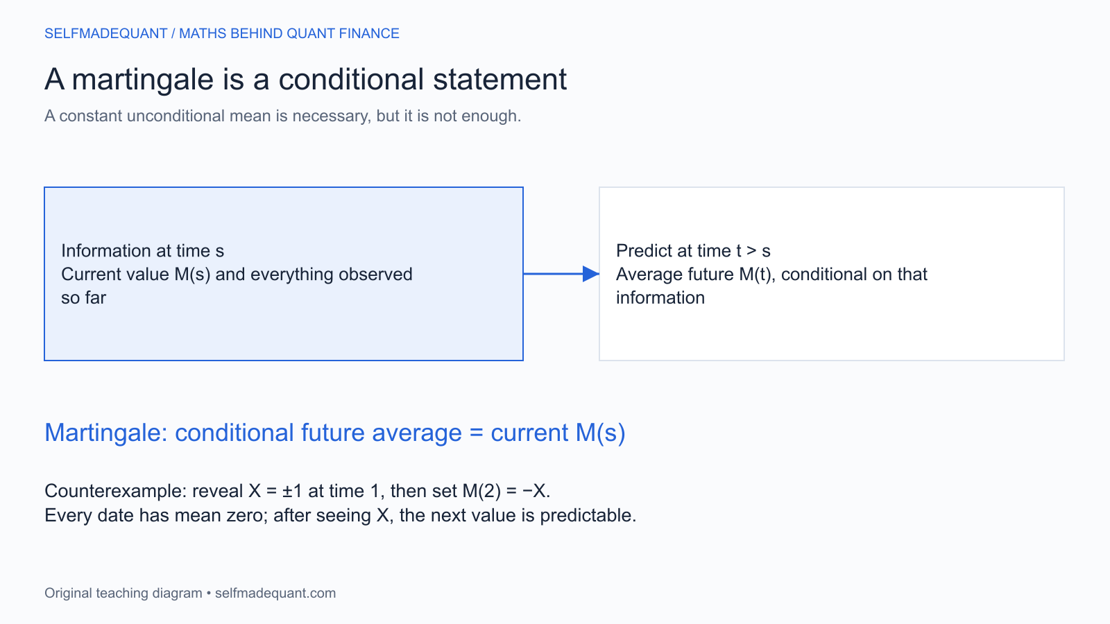
Take a fair random variable $X\in\{-1,1\}$ . Set $M_0=0$ , reveal $X$ at date 1, define $M_1=X$ , and set $M_2=-X$ .

Every date has unconditional mean zero. But once $X$ is observed,

\mathbb E[M_2\mid\mathcal F_1]=-X\ne X=M_1.

The date-2 value is completely predictable from the date-1 observation. The process fails the martingale condition even though a chart of its cross-sectional mean would be flat.

This is a practical simulation lesson. Checking that an estimated discounted stock mean matches today’s price is useful, but it checks only one unconditional implication. It cannot certify every conditional expectation in the model. Conditional checks can group continuations by a known current state, provided the grouping and simulation are consistent with the model.

For practice translating observations into conditional distributions, use the conditional probability interview questions. The same discipline applies: specify what was observed before calculating the average.

Brownian motion supplies a continuous-time example

For standard Brownian motion $W_t$ , future increments $W_t-W_s$ are independent of the past and have mean zero. With its usual information flow,

\mathbb E[W_t\mid\mathcal F_s] =W_s+\mathbb E[W_t-W_s\mid\mathcal F_s]=W_s.

The process $W_t$ is a martingale. Its square is not: independent Gaussian increments give

\mathbb E[W_t^2\mid\mathcal F_s]=W_s^2+(t-s).

Consequently $W_t^2-t$ is a martingale. Subtracting time compensates for the expected accumulation of squared noise.

Similarly, if $X_t=x+\mu t+\sigma W_t$ with constant coefficients, the compensated process $X_t-\mu t$ is a martingale. The original process generally has drift. The exception is $\mu=0$ .

These examples connect directly to Brownian motion and quadratic variation, then to Itô’s lemma. The square example is an early sign that ordinary differentiation will miss something.

The exponential correction

A more financially useful example is

Z_t=\exp\left(\sigma W_t-\tfrac12\sigma^2t\right)

for a constant $\sigma$ . Why subtract the variance term? A zero-mean Gaussian $G$ with variance $v$ satisfies $\mathbb E[e^{aG}]=e^{a^2v/2}$ . Exponentiation increases the average because it is convex. The correction offsets that increase.

Write $Z_t$ in terms of its current value:

Z_t=Z_s\exp\left(\sigma(W_t-W_s)-\tfrac12\sigma^2(t-s)\right).

The second factor has conditional mean one, so $\mathbb E[Z_t\mid\mathcal F_s]=Z_s$ . This proof establishes the martingale property for this constant-coefficient exponential on finite horizons; it does more than observe a zero drift symbol in a stochastic differential equation.

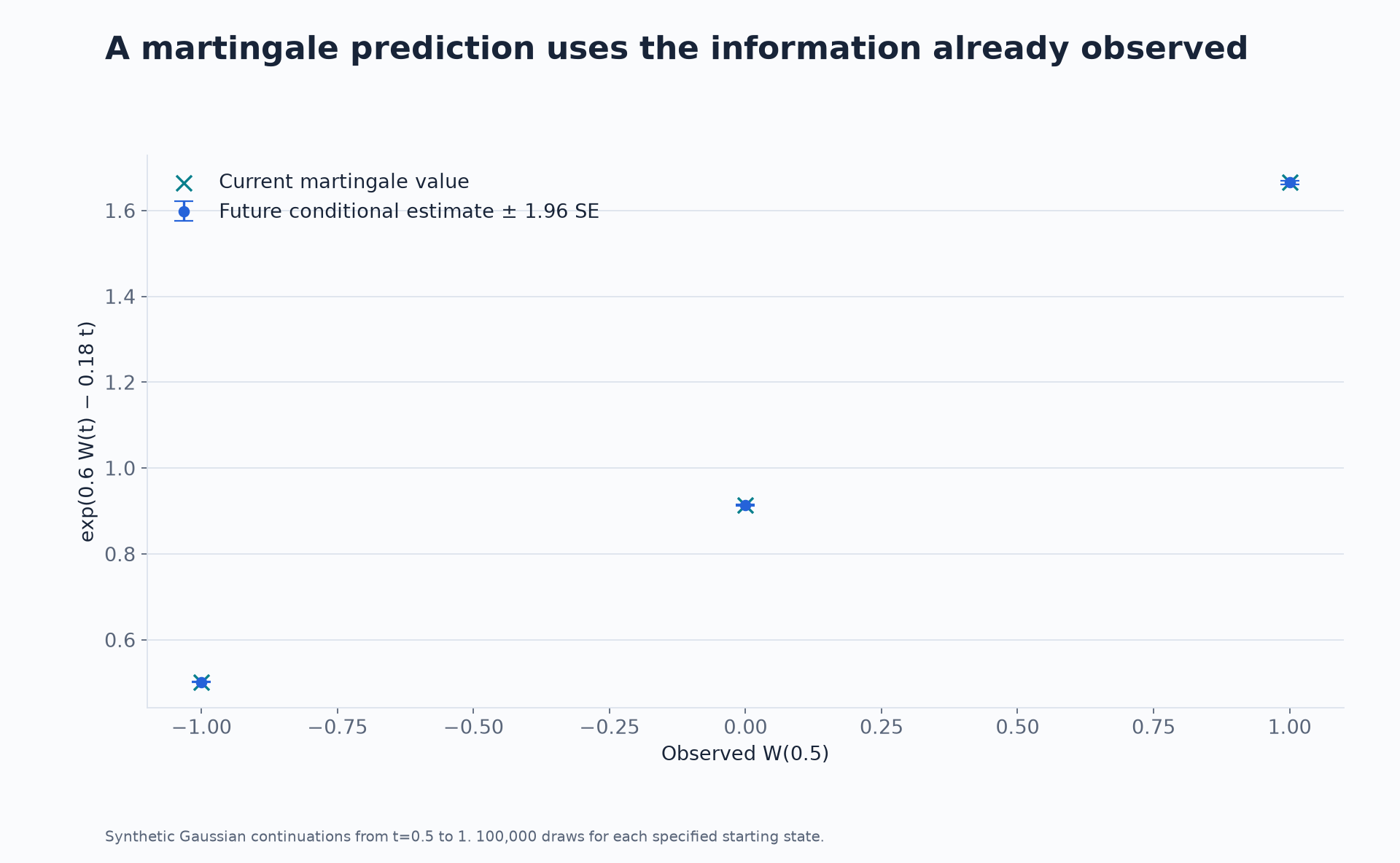
Conditional Monte Carlo averages of the exponential Brownian martingale agree with its current values within displayed sampling uncertainty

The chart fixes time $s=0.5$ and three possible Brownian states. Each experiment draws 100,000 independent continuations to time 1. The error bars describe finite simulation uncertainty. These are synthetic continuations from specified states, not historical stock-price observations.

For general stochastic integrals, “zero drift” initially identifies a local martingale under suitable conditions. A local martingale is a broader technical class; additional integrability conditions are needed to conclude that it is a true martingale. Do not extend the constant-coefficient result to every stochastic-volatility model without checking those conditions.

What is a martingale in risk-neutral pricing?

Suppose a stock follows constant-coefficient geometric Brownian motion, pays no dividends, and the continuously compounded risk-free rate is

r

. Under a risk-neutral measure

\mathbb Q

S_t=S_0\exp\left((r-\tfrac12\sigma^2)t+\sigma W_t^{\mathbb Q}\right).

Then $e^{-rt}S_t=S_0Z_t$ is a martingale under $\mathbb Q$ . Discounting removes the risk-free growth, and the exponential correction handles the noise.

This does not say that the stock’s expected return in the physical world is $r$ . Under a forecasting measure $\mathbb P$ , its modelled drift might be $\mu$ . Pricing and forecasting use different expectations for different purposes.

Dividends require care. With continuous proportional dividend yield $q$ , the ex-dividend stock has risk-neutral drift $r-q$ . Its discounted ex-dividend price alone is generally not a martingale. The discounted gains process, including dividends received, is the relevant object; equivalently, the discounted value of a strategy that reinvests the dividends has the martingale property in this model.

The two-state risk-neutral pricing example shows where pricing weights come from without assuming stochastic calculus. For the continuous model, Black–Scholes links the same idea to replication.

Does stopping a fair game create an advantage?

Suppose you play the fair walk for at most three rounds and stop early if you reach $+1$ . The stopping time is bounded. The optional-stopping theorem applies to this discrete-time integrable martingale and gives expected stopped value zero.

The paths that reach the profit target do not tell the whole story. Some paths finish the third round with a loss. An evaluation that counts successful exits while omitting unfinished or losing games changes the experiment.

The doubling-after-losses system makes the same omission easy to hide. After a loss, double the next stake so that a future win recovers the accumulated losses and adds one unit. A long losing run then demands an exponentially large stake. Removing a maximum stake and a final stopping date does not justify applying a bounded-stopping theorem to the resulting limiting strategy. Finite bankrolls and borrowing limits matter even before that mathematical issue.

The word “martingale” in the strategy’s name is not a proof of profitability. For a bounded worked stopping problem, see expected value and waiting-time interview questions.

A checkpoint before moving on

Consider $X_t=W_t+2t$ . Is it a martingale? No: conditional expected future value is $X_s+2(t-s)$ . Subtracting $2t$ recovers Brownian motion and the martingale condition.

Now consider $Y_t=W_t^2$ . Its unconditional mean is $t$ , and its conditional drift over $[s,t]$ is also $t-s$ . The compensated quantity $Y_t-t$ is the martingale. These two examples distinguish deterministic drift compensation from the correction created by squaring random increments.

For a first pass, remember the three things to state: the random process, the information available, and the probability measure. Then calculate a conditional expectation rather than relying on a flat average chart.

Sources and further study

MIT’s Advanced Stochastic Processes lecture notes provide a rigorous continuation through filtrations, martingales and stopping. The examples, simulations and diagrams above were constructed for this article.