One option, five pricing methods: a reproducible Python lab
A formula, a tree, a simulation, and a Fourier integral should not be compared by changing the contract every time.
In this Python option-pricing lab, we hold the European payoff and geometric Brownian motion (GBM) assumptions fixed. We compare Black–Scholes, a Cox–Ross–Rubinstein binomial tree, Monte Carlo, Fourier quadrature and FFT pricing. After that, we make one controlled contract change: allowing early exercise of a put.
The point is to distinguish numerical error, exercise value, and model assumptions. A smaller solver error does not establish a better market model, and a model value does not establish an executable trading opportunity.
Define the experiment
We price one call per underlying unit with spot and strike , one year to expiry, continuously compounded rate 5%, continuous dividend yield 2%, and annual volatility 20%. The Monte Carlo seed is 20261007.
pricing_lab.py, requirements.txt, a README, executed results.json, and eight generated figures. It uses synthetic data only. There is no historical option chain, calibration, backtest, or claim of investment profitability.Run the project in an environment with NumPy, SciPy, and Matplotlib. The lab writes results relative to its own location, so extracting the reader bundle preserves the experiment's paths. The version record documents the environment used for these published results.
The implementations are intentionally readable. They cover a dividend-adjusted BSM formula, recombining CRR tree, exact-terminal GBM Monte Carlo, antithetic Monte Carlo, Carr–Madan quadrature, and a grid FFT. The last two share the same characteristic function.
Python option-pricing results: Black–Scholes, binomial, Monte Carlo and Fourier
| Method | Call value | Relevant uncertainty or error |
|---|---|---|
| BSM formula | $9.2270055082 | Benchmark under the stated model |
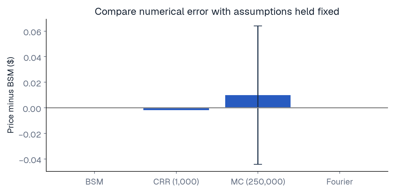
| CRR, 1,000 steps | $9.2250617378 | Error of about −$0.001944 |
| Plain MC, 250,000 evaluations | $9.2368995790 | Estimated SE $0.027629 |
| Antithetic MC, equal evaluation budget | $9.2190912097 | Estimated SE $0.020456 |
| Carr–Madan quadrature | $9.2270055082 | Agreement to numerical precision in this case |
| FFT with strike interpolation | $9.2333347211 | Error of about +$0.006329 |
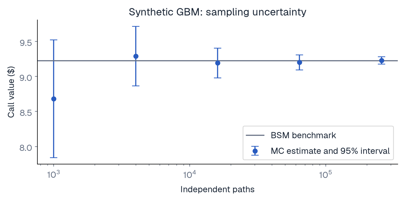
The plain Monte Carlo approximate 95% interval is . The antithetic interval is . Both contain the benchmark for this fixed seed. That is a recorded outcome, not a requirement that every correctly implemented interval must contain the true value.
Antithetic Monte Carlo uses 125,000 independent pair means, requiring 250,000 terminal payoff evaluations. Its estimated standard error is about 26% lower than plain simulation in this experiment. We compare equal terminal evaluation budgets; runtime may still differ because implementations and hardware differ.
Binomial tree convergence to Black–Scholes
The CRR construction tends toward the GBM diffusion as its time steps become small. Its vanilla payoff is discounted backwards using the same carry assumptions as BSM. We therefore expect convergence to the same European price.
The finite tree represents the payoff kink on a discrete terminal grid. Odd and even step counts can show different errors. The lab plots those errors and checks a 2,000-step value against a specified tolerance. Do not judge convergence by displaying two rounded values that happen to look identical.
For the American put, backward induction adds the exercise maximum. On the 1,000-step tree, the European put is and the American put is . The difference is about under this grid and model.
That difference has a different meaning from the call tree's discrepancy against BSM. We changed the holder's rights. The American put is a different contract. Compare its price with the European put on the same grid to isolate the exercise feature as clearly as possible.
Monte Carlo standard error and the martingale check
Exact GBM terminal simulation draws the correct terminal distribution, but the sample mean still fluctuates. Increasing independent observations shrinks its standard error at the usual square-root rate. It does not alter the model's assumed volatility.
Antithetics average each payoff with its payoff. The pair is one independent observation. Treating both members as independent would misstate the interval. The lab makes the observation count and terminal evaluation count explicit in the output.
The benchmark being inside an interval is only one diagnostic. Also verify expected stock carry, payoff construction, discounting, and independent draws. A single random seed can hide a mistake or reveal an unusually large fluctuation; it cannot prove estimator correctness by itself.
Why quadrature and FFT differ
Both invert the same damped transform. Adaptive quadrature targets the requested strike directly. The FFT computes an evenly spaced log-strike grid, and our strike requires interpolation.
The current FFT grid uses 4,096 points, frequency spacing 0.05, damping 1.5, and log-strike spacing about 0.03068. Refinement affects truncation and interpolation together. A production solver needs explicit tolerances across the relevant region, not only at the benchmark strike.
Quadrature matches BSM here and remains stable when damping changes among 0.5, 1.0, and 2.0 and the integration limit is increased. The lab also checks five strikes. The routine's local error estimate does not quantify the economic uncertainty in the model.
Read the checks as evidence with a scope
The executed run passes nine checks: European parity, tree convergence, American put dominance, quadrature agreement, damping stability, a strike-grid comparison, FFT accuracy at the stated tolerance, recorded fixed-seed Monte Carlo coverage, and expiry/zero-volatility boundaries.
These are benchmark checks for a teaching implementation. They do not validate a production risk system across arbitrary parameter regimes. In particular, the lab does not implement local volatility, Heston simulation, jump calibration, continuous barrier corrections, or least-squares Monte Carlo. The earlier articles explain where those extensions belong.
Good validation combines independent identities with limiting cases and an external or analytically known benchmark. Merely duplicating the implementation in a test would give less useful evidence. A production extension should add the tests that its new contract and model demand.
Extend one axis at a time
First vary tree steps. Then vary Monte Carlo paths while keeping the terminal model exact. Then vary FFT grid parameters. Record the resulting errors separately.
Next change volatility while retaining the BSM formula. That targets input sensitivity. Finally change the contract's exercise rule on the tree. That targets economic rights. Keeping those experiments distinct makes the results interpretable.
To explore path dependence, add an arithmetic Asian payoff with a stated observation schedule and a control variate. To explore richer dynamics, begin with a separately validated characteristic function or simulation scheme. Compare limiting cases before attempting calibration.
Choosing a method is choosing a task
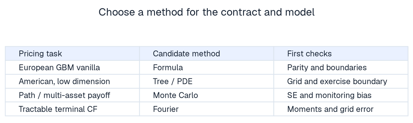
Closed-form BSM is an excellent vanilla benchmark when its assumptions apply. A tree is useful for low-dimensional exercise decisions. Monte Carlo is flexible for complex path and multi-asset payoffs, with sampling and discretization work to manage. Fourier methods are attractive for terminal payoffs when a tractable characteristic function is available, especially across many strikes. Finite-difference PDE methods are another important family for low-dimensional state problems and exercise boundaries; they sit beyond this lab's implemented scope.
The right method is the one that represents the contract, works with the chosen model, and achieves a controlled error within the available budget. No algorithm wins every pricing problem.
Continue learning
Sources and reproducibility
Go deeper with lessons, derivations and worked exercises behind this article.