Geometric Brownian motion: solution, moments and Python simulation

Published 15 October 20265 min readThe maths behind quant finance:Part 1 Part 2 Part 3Part 4Part 5 Part 6

Geometric Brownian motion, or GBM, is a positive-price diffusion with constant proportional drift and volatility. Its defining equation is $dS_t=\mu S_tdt+\sigma S_tdW_t$ , and its exact solution is an exponential of Brownian motion.

It is useful because we can solve its distribution, simulate exact transitions at observation dates, and benchmark option-pricing code. It is also limited: constant volatility and continuous paths leave out important features of real markets.

The first distinction to learn is between price growth and log-price growth. With 8% arithmetic drift and 30% volatility, expected log growth is 3.5% per year. Both numbers can be correct in the same model.

This article derives that result, calculates moments, and compares exact simulation with Euler stepping. For the calculus behind the solution, read Itô’s lemma.

The model and its units

Assume $S_0>0$ and constant $\mu$ and $\sigma\geq0$ . Under a specified probability measure,

\frac{dS_t}{S_t}=\mu\,dt+\sigma\,dW_t.

Here $\mu$ is the instantaneous proportional drift. If time is measured in years, it has units per year. Volatility $\sigma$ is quoted per square-root year, so $\sigma\,dW_t$ is dimensionless like a proportional price change.

“Geometric” indicates that the noise scales with the current level. A ten-unit price movement is much larger proportionally for a stock at 20 than for one at 200. GBM makes the distribution of future price ratios independent of the current absolute price level when coefficients are constant.

The symbol $\mu$ does not specify the measure by itself. Under a physical forecasting model, it represents an assumed expected return. Under a risk-neutral pricing model for a stock with continuous dividend yield $q$ , replace it with $r-q$ . Label that choice before generating draws.

Solve it by taking logarithms

For $f(s)=\log s$ , Itô’s lemma gives

d\log S_t=(\mu-\tfrac12\sigma^2)dt+\sigma\,dW_t.

Integrate from zero to $t$ and exponentiate:

S_t=S_0\exp\left((\mu-\tfrac12\sigma^2)t+\sigma W_t\right).

The solution remains strictly positive at every finite time. For $\sigma>0$ , its logarithm is normally distributed, so its price is lognormally distributed:

\log(S_t/S_0)\sim N\left((\mu-\tfrac12\sigma^2)t,\sigma^2t\right).

A common error is to use $\mu t+\sigma W_t$ in the exponent. That produces expected price $S_0e^{(\mu+\sigma^2/2)t}$ , which is a different model. The correction is needed to preserve the drift stated in the original equation.

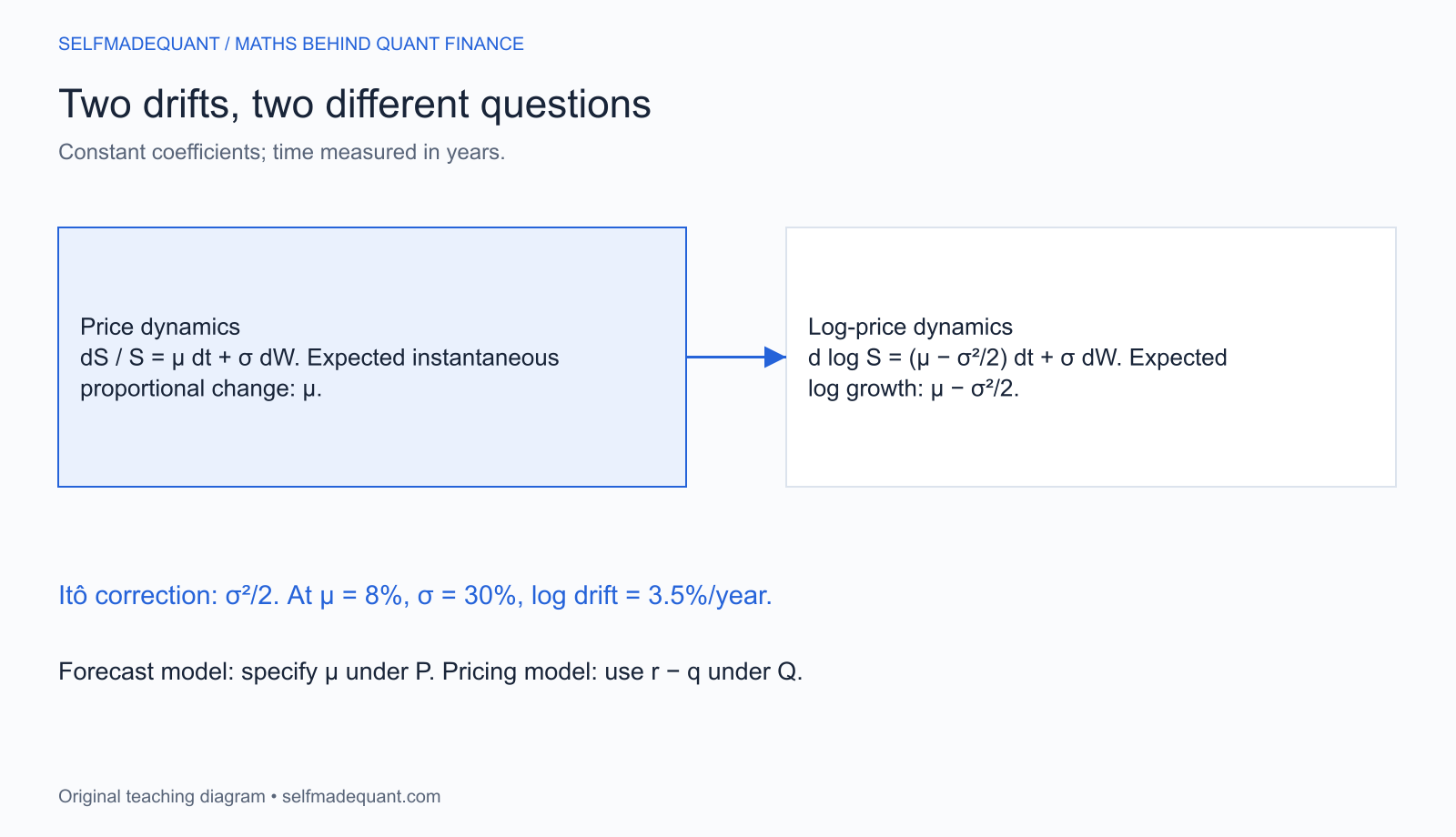
The proportional price drift and the log-price drift differ by half the variance rate; the probability measure determines which price drift to use

Mean, median and expected log return

The Gaussian exponential identity gives

\mathbb E[S_t]=S_0e^{\mu t},\qquad \operatorname{median}(S_t)=S_0e^{(\mu-\sigma^2/2)t}.

The mean exceeds the median when volatility and horizon are positive. High-price outcomes stretch the right tail of the lognormal distribution and pull up the mean. The median is the point with half the terminal distribution below it; it is not a claim that every path follows a smooth median curve.

Expected log return is $(\mu-\sigma^2/2)t$ . Expected simple return over the horizon is $e^{\mu t}-1$ . The instantaneous drift $\mu$ equals neither horizon quantity exactly for an arbitrary horizon, although the simple-return expression is approximately $\mu t$ for small $t$ .

For $S_0=100$ , $\mu=0.08$ , $\sigma=0.30$ and $t=5$ ,

\mathbb E[S_5]=100e^{0.4}\approx149.18,\qquad \operatorname{median}(S_5)=100e^{0.175}\approx119.12.

import math

s0, mu, sigma, years = 100.0, 0.08, 0.30, 5.0
print(f"mean={s0 * math.exp(mu * years):.2f}")
print(f"median={s0 * math.exp((mu - sigma**2 / 2) * years):.2f}")
# mean=149.18
# median=119.12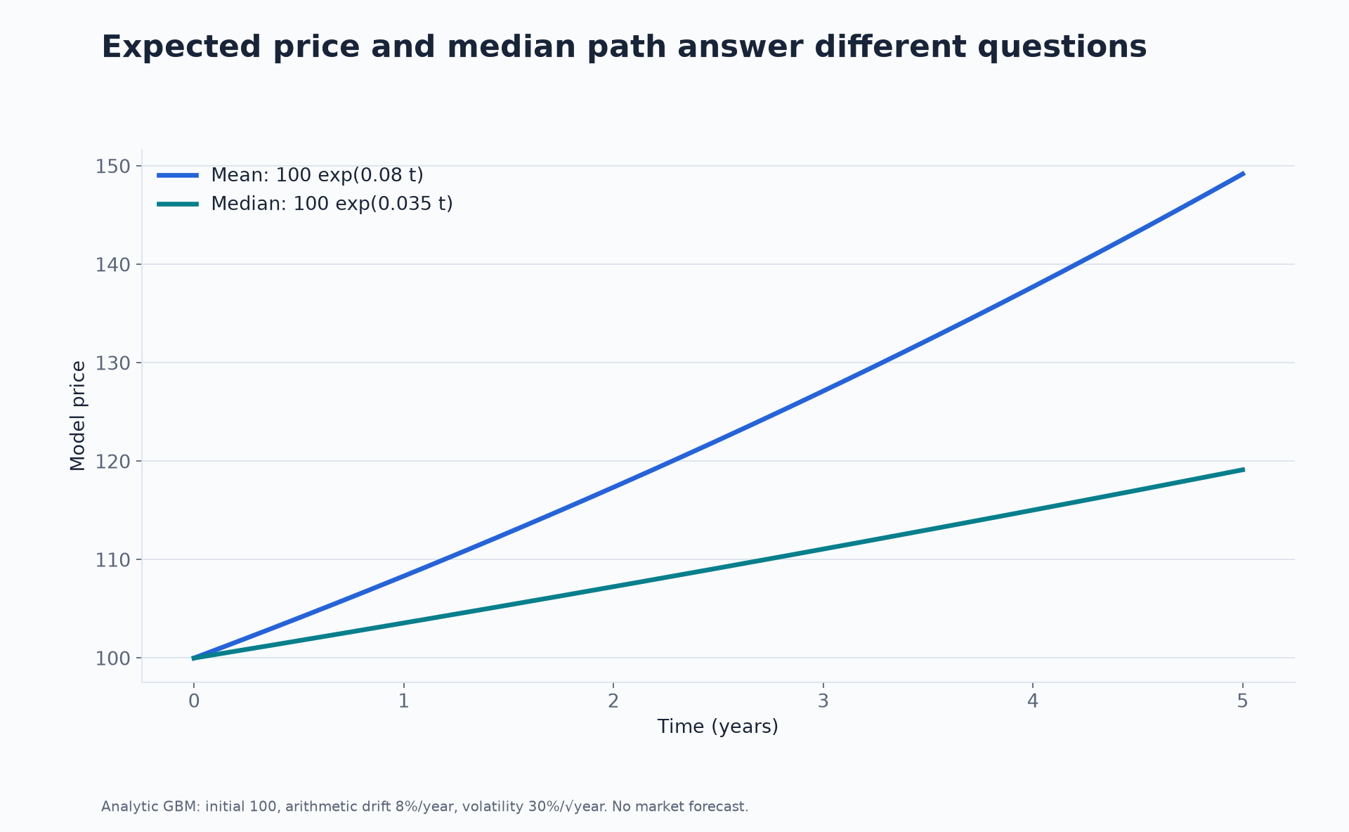

Analytic GBM mean and median curves diverge over five years for 8 percent drift and 30 percent annualised volatility

The variance is

\operatorname{Var}(S_t)=S_0^2e^{2\mu t}\left(e^{\sigma^2t}-1\right).

You can derive it by calculating $\mathbb E[S_t^2]=S_0^2e^{(2\mu+\sigma^2)t}$ and subtracting the squared mean. Setting $\sigma=0$ reduces the variance to zero and recovers deterministic exponential growth, a useful boundary check.

The gap between arithmetic and log growth is sometimes called a volatility drag in discussions of compounding. Here it is an exact model identity. It does not establish an empirical forecast or a universal realised penalty across all return processes.

Exact simulation at chosen dates

Over an interval of length $h$ , conditional on the current price,

S_{t+h}=S_t\exp\left((\mu-\tfrac12\sigma^2)h+\sigma\sqrt h Z\right),\qquad Z\sim N(0,1).

Use independent $Z$ values across disjoint intervals. For paths on a grid, form cumulative log increments and exponentiate. For a European payoff that depends only on $S_T$ , draw the terminal distribution directly; there is no need to allocate an entire daily path.

import numpy as np

rng = np.random.default_rng(20261015)
s0, mu, sigma, horizon = 100.0, 0.08, 0.30, 1.0
z = rng.standard_normal(200_000)
terminal = s0 * np.exp((mu - sigma**2 / 2) * horizon
                       + sigma * np.sqrt(horizon) * z)
print(f"sample mean={terminal.mean():.2f}")
print(f"theory mean={s0 * np.exp(mu * horizon):.2f}")
print(f"all positive={bool(np.all(terminal > 0))}")
# sample mean=108.38
# theory mean=108.33
# all positive=True

The sample mean need not equal the theoretical mean. Its standard error is the sample price standard deviation divided by the square root of the number of independent draws. Treat an unexpectedly large difference as a diagnostic, while allowing normal sampling fluctuations.

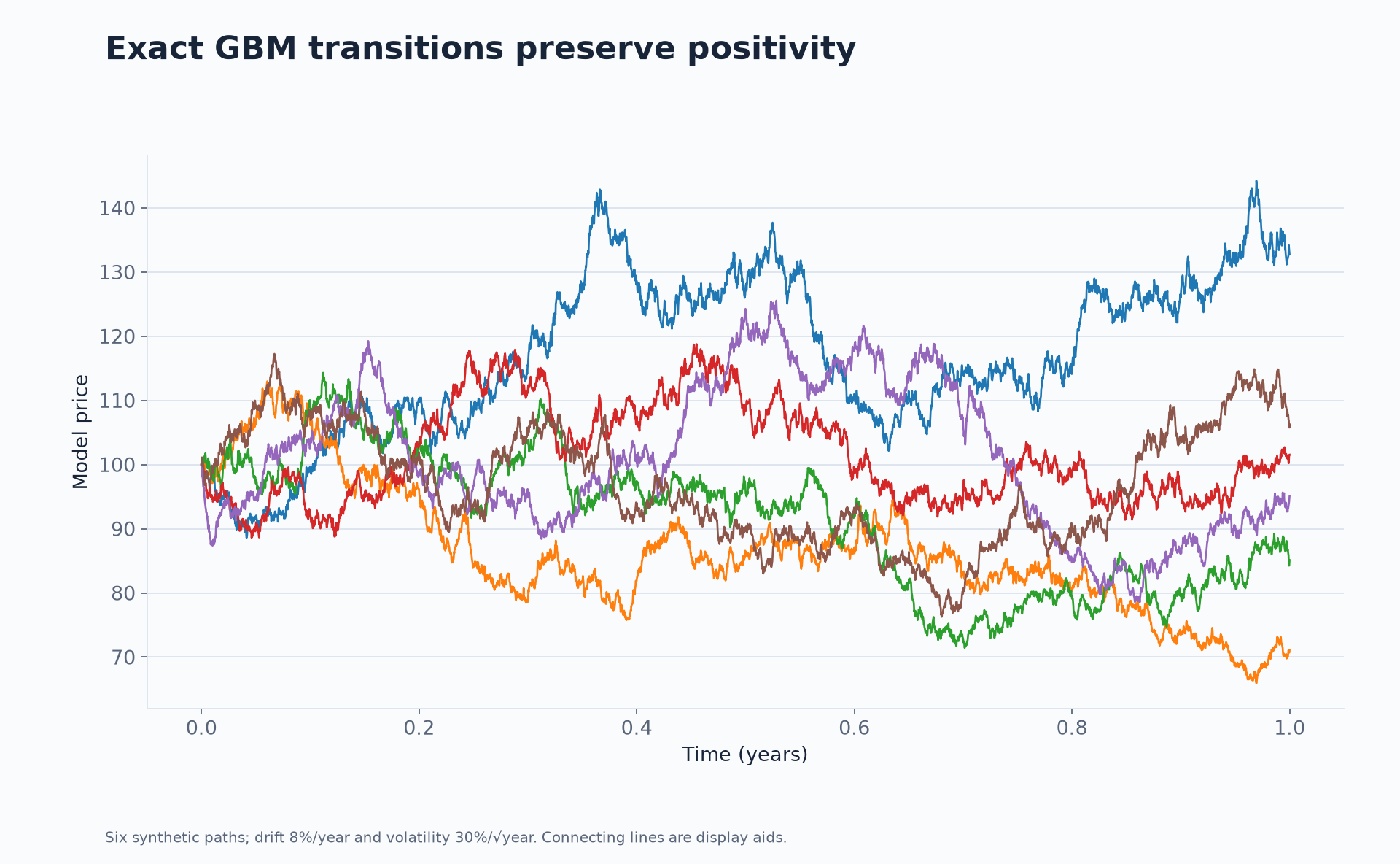
Six synthetic geometric Brownian paths stay positive when sampled using the exact exponential transition with fixed drift and volatility

“Exact transition” means the chosen grid values have the specified model distribution. It does not mean the model is exact for markets, the sample mean has no error, or a line drawn between observations detects all continuous-time barrier events.

Why Euler can produce a negative price

Euler stepping uses

S_{t+h}^{\mathrm E}=S_t^{\mathrm E}(1+\mu h+\sigma\sqrt h Z).

When the current value is positive, the next value is negative if

Z<-\frac{1+\mu h}{\sigma\sqrt h}.

A Gaussian variable has an unbounded lower tail, so for $\sigma>0$ this event has positive probability for any positive finite step. At small daily steps and moderate volatility, the probability may be extremely small; at large steps it becomes easier to observe.

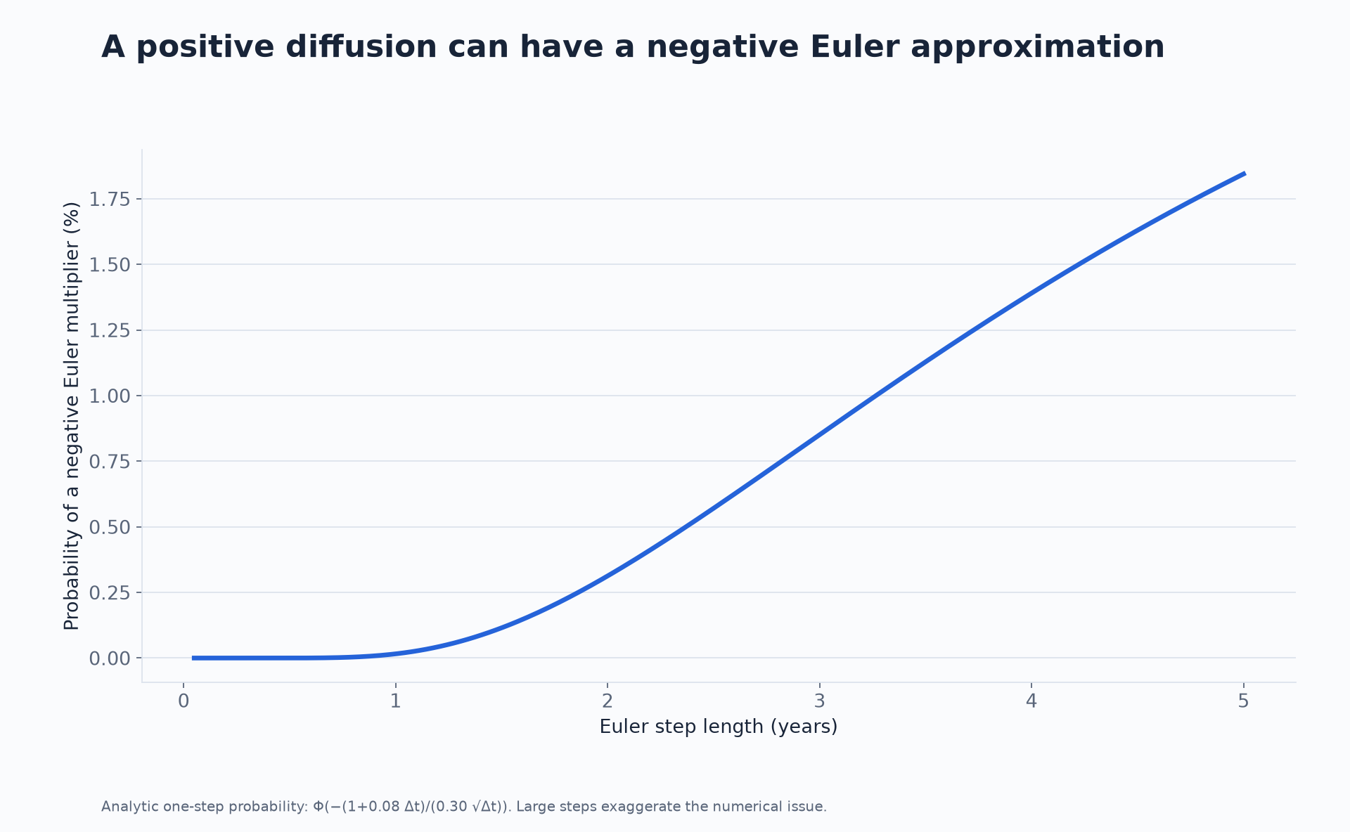
Analytic probability of a negative one-step Euler multiplier increases over the displayed large time steps, although the underlying exact GBM remains positive

Clipping negative prices to zero changes the approximation and can introduce a different bias. If the exact GBM transition is available, using it is simpler. For more general stochastic differential equations, the numerical scheme and its convergence properties need their own analysis.

When comparing schemes, use common Brownian increments where possible. Otherwise unrelated noise can obscure the discretisation difference you are trying to measure. A simulation can have both sampling error and time-step bias; raising the path count addresses only the first.

Pricing measure versus forecasting measure

Suppose your forecasting assumption is an 8% stock drift. A risk-neutral European option calculation with $r=3\%$ and no dividends uses 3% in the stock dynamics. That change is required by the pricing framework, rather than a claim that your forecast was wrong.

Under $\mathbb Q$ with constant dividend yield,

\mathbb E^{\mathbb Q}[S_T]=S_0e^{(r-q)T}.

For

q=0

, the discounted stock is a martingale. With dividends, use the discounted gains or reinvested-total-return process rather than the ex-dividend stock alone.

The risk-neutral pricing article derives the principle in two states. The Monte Carlo option-pricing article then uses exactly this terminal GBM transition, adds discounting and reports an error bar.

Where the model is useful, and where to challenge it

GBM is a strong teaching and implementation benchmark. Its known moments and analytic European option price let you check whether a simulation, discount factor and payoff implementation agree under a shared model.

It is a weak basis for assuming every future market scenario is covered. Constant volatility excludes volatility clustering and changing regimes. Continuous paths exclude jumps. Normal log returns impose particular tail behaviour. A single constant rate and dividend yield may not fit the contract’s actual cash flows.

Parameter estimation adds another issue: drift is difficult to infer precisely from noisy returns. Simulating millions of paths around a poorly supported drift assumption does not make that assumption more accurate. In risk work, distinguish uncertainty about the distribution from numerical uncertainty conditional on it.

For portfolios, dependence assumptions matter alongside each individual GBM. Marginal distributions alone do not determine basket risk or basket option value. For pricing, matching one option does not ensure a constant-volatility model matches the whole implied-volatility surface.

Download and study next

The series code package reproduces the paths, moments and Euler comparison. It also includes the Monte Carlo estimation experiment and the European option benchmark, so you can follow the same assumptions through several calculations.

Use the Options Pricing programme to study the financial context and the stochastic-processes lesson for the mathematical bridge. If implementation is the obstacle, start with Python for quant finance beginners.

Sources and further study

MIT’s 2024 mathematics-with-finance course materials provide further Itô-calculus study. NumPy’s Generator documentation documents the simulation interface. All parameters above are illustrative, and all displayed model moments follow from the stated constant-coefficient GBM.