Black–Scholes: why the expected stock return leaves the price

You expect a stock to earn 12% a year. Someone else expects 7%. Under the same constant-volatility Black–Scholes assumptions, you can still agree on the price of its European call.

That sounds odd if you think option pricing means forecasting a payoff and discounting it. The missing step is hedging. A dynamically adjusted stock position removes the model's instantaneous stock risk. The resulting locally riskless portfolio must earn the financing rate. The stock's expected return disappears from the pricing equation.

The conclusion depends on a demanding trading model. It does not mean expected returns are irrelevant to investment decisions, or that an actual option can be perfectly hedged with occasional trades.

The derivation connects three ideas: Itô's lemma describes how an option changes when its stock follows Brownian motion; delta hedging removes the instantaneous random term; risk-neutral valuation expresses the same price as an expectation. We will use each step to explain the Black–Scholes formula rather than treating it as a lookup rule.

Geometric Brownian motion: the Black–Scholes stock model

Take an ex-dividend stock with continuous yield $q$. Under the real-world measure, suppose:

Here $\mu$ is the drift of the ex-dividend price, $\sigma$ is a constant annual volatility, and $W$ is Brownian motion. Rates and yield are deterministic constants in this article. Trading is continuous and frictionless, borrowing and lending use the same rate, and the stock can be traded in arbitrary quantities. The stock follows continuous paths.

Itô's lemma: the stochastic chain rule

Itô's lemma, also called Itô's formula, is the chain rule used in stochastic calculus for functions of diffusion processes. For $dX_t=a_tdt+b_tdW_t$ and a function $f(x,t)$ with one continuous time derivative and two continuous space derivatives:

For a European option let $V(S,t)$ be its value, smooth before expiry in this model. Applying Itô's lemma gives:

The curvature term involves gamma, $V_{SS}$. Applying the ordinary chain rule and dropping that term would lose the contribution of stock variance to option value.

Delta hedging derives the Black–Scholes PDE

Choose a hedge of $\Delta=V_S$ shares. The stock component has random change $\Delta\sigma S\,dW$, matching the option's random change. A self-financing replication also accounts for stock dividends $qS\Delta dt$ and the financing of the remaining position. Equating the hedged cash flows yields:

This is the Black–Scholes pricing PDE. Its terminal condition specifies the contract: $V(S,T)=(S-K)^+$ for a call. The PDE alone is not a price until boundary and terminal conditions are supplied.

The terms have financial meanings. $V_t$ describes calendar-time change. Curvature $V_{SS}$ interacts with variance. $(r-q)SV_S$ incorporates risk-neutral carry. $rV$ is the financing requirement. The real-world drift $\mu$ has cancelled.

Risk-neutral valuation and the martingale condition

For constant $r$, $q$ and $\sigma$, the dividend-reinvested discounted stock $M_t=e^{-(r-q)t}S_t$ is a martingale under $\mathbb Q$. Thus $\mathbb E^{\mathbb Q}[M_T\mid\mathcal F_t]=M_t$. This does not assert that a stock earns the risk-free rate under real-world probabilities. It describes the pricing measure consistent with replication in this model.

To find the terminal distribution, apply Itô's lemma again, now to $f(S)=\log S$. Since $f_S=1/S$ and $f_{SS}=-1/S^2$:

Over a remaining horizon $\tau=T-t$, the terminal stock is therefore lognormal:

The Black–Scholes formula: what d1 and d2 mean

Integrating the discounted call payoff over that distribution gives:

$\Phi$ is the standard normal cumulative distribution function. The put follows from parity, or from integrating its own payoff:

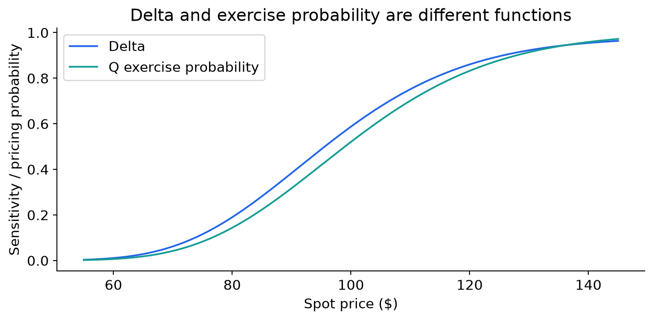
A subtle distinction matters. $\Phi(d_2)$ is the risk-neutral probability that the call finishes in the money in this model. $\Phi(d_1)$ enters the stock-weighted expectation; it is not the same probability. Call delta is $e^{-q\tau}\Phi(d_1)$, and delta is a sensitivity, not a general probability forecast.

Work one price all the way through

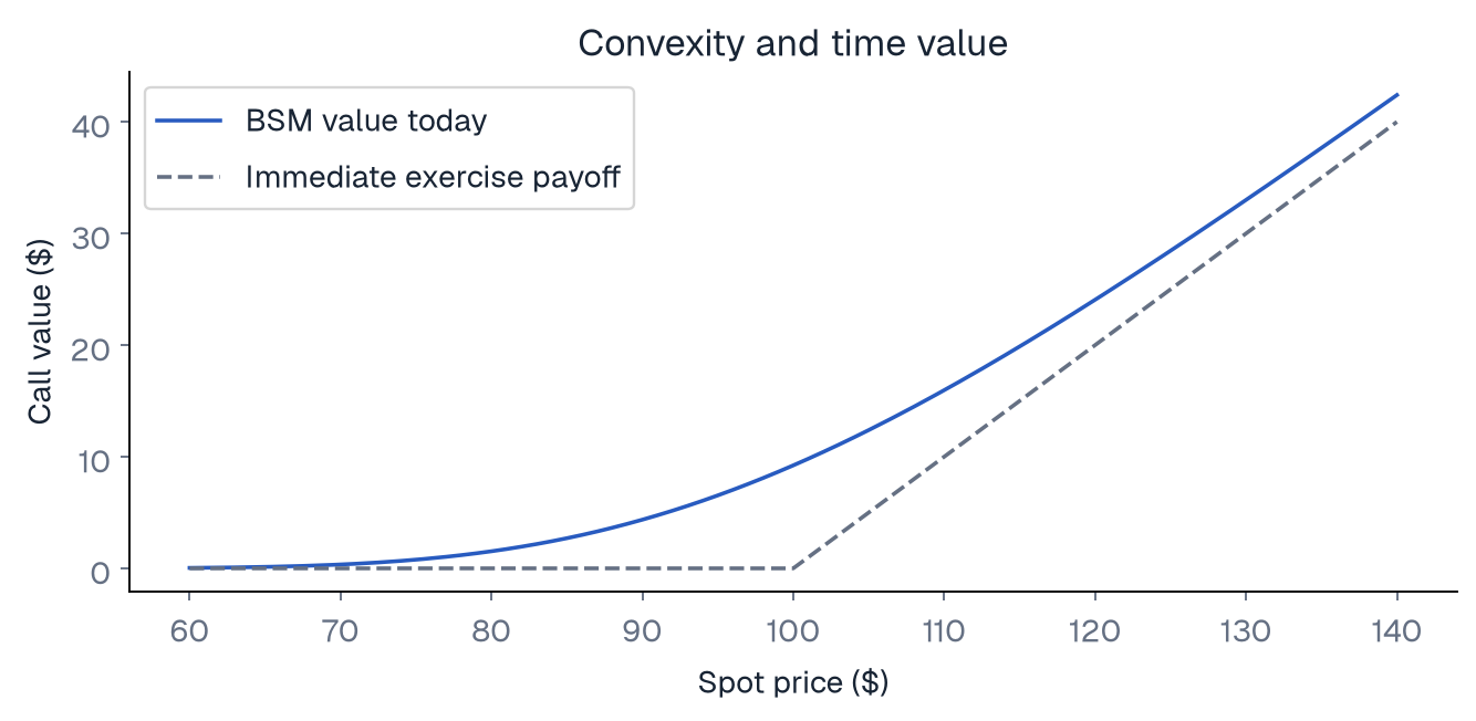
Our common inputs are $S=K=100$, $\tau=1$, $r=0.05$, $q=0.02$, and $\sigma=0.20$. Then $d_1=0.25$ and $d_2=0.05$. The call price is approximately $9.2270$, and the put price is approximately $6.3301$.

The difference is $2.8969$, matching $100e^{-0.02}-100e^{-0.05}$. The price lies between its no-arbitrage bounds. Those independent identities are more useful than copying the number into a second implementation with the same mistake.

Using a maturity of 365 in a function expecting years will produce nonsense while leaving the code perfectly valid. So will supplying 20 for a volatility intended as 0.20. Record units at the interface: years, annual rate decimals, annual volatility decimals, and a consistent currency per underlying unit.

Option Greeks: delta, gamma and vega

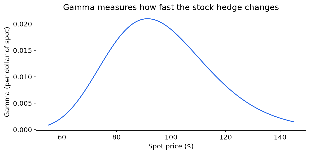
The call's delta is its first spot derivative. Gamma is the second:

$\varphi$ is the standard normal density. Gamma tells us how quickly delta changes as spot moves. A short option is short convexity: its stock hedge needs adjustment as the underlying changes. Perfect cancellation relies on the continuous-trading limit.

Vega is:

This derivative measures change per 1.00 change in volatility, not per one percentage point. Divide by 100 for the usual one-vol-point convention. Always state the convention when comparing systems.

Greeks are local approximations. A delta-only estimate can miss a large move, a volatility change, or a discontinuity in payoff. Even a detailed Greek expansion remains tied to a chosen model and the size of the move.

Implied volatility reverses the calculation

Observed option prices can be mapped to the volatility that makes the BSM formula reproduce them. That is implied volatility. It is a quote transformation, not proof that the market follows constant-volatility GBM.

Across strikes and expiries, the resulting surface is usually not flat. A single constant volatility cannot match all those prices simultaneously. Some quotes may have little vega, making the inversion poorly conditioned. Midpoint quotes, stale prices, and inconsistent forwards can also distort the result.

Try it

Set $q=0$ while keeping the other benchmark inputs fixed. Predict the direction of the call change before running the lab: lower dividend yield increases the forward and raises the call price. Then compute parity with the changed yield. It must still hold.

Continue learning

Sources