Monte Carlo simulation in finance: a beginner’s guide with Python

Published 15 October 20266 min readThe maths behind quant finance:Part 1 Part 2 Part 3 Part 4 Part 5Part 6

Monte Carlo simulation estimates a quantity by drawing random outcomes from a specified model and averaging the relevant calculation. In finance, the target might be an expected loss, a derivative payoff, an exposure or a probability of breaching a limit.

The method does not decide which model is appropriate. It estimates what that model implies. A useful result therefore states the quantity being estimated, the distribution used, the number of independent observations and a measure of sampling uncertainty.

We will calculate an expected reserve shortfall that has an exact answer, reproduce it with Python, and explain the error bar. For option pricing under a risk-neutral distribution, use the separate Monte Carlo option-pricing guide. This page teaches the general estimation method.

Start with the target, not the random generator

Imagine a toy one-period loss $L$ with four possible outcomes. This is an illustrative physical risk model, with fixed inputs rather than estimated market data.

Loss	Probability	Shortfall above a reserve of 12
0	0.50	0
10	0.30	0
30	0.15	18
80	0.05	68

We want $\theta=\mathbb E[(L-12)^+]$ , the expected amount by which loss exceeds the reserve. Exact enumeration gives

\theta=0.15\times18+0.05\times68=6.10.

Expected loss itself is $0.3\times10+0.15\times30+0.05\times80=11.50$ . Taking the shortfall of that expected loss gives $(11.50-12)^+=0$ , which is different from 6.10.

The difference is nonlinearity: averaging losses first and applying the positive-part function afterward changes the target. For nonlinear payoffs and risk measures, preserving the order of operations is essential.

The Monte Carlo estimator

Draw independent losses $L_1,\ldots,L_N$ from the stated distribution, calculate $Y_i=(L_i-12)^+$ , and average:

\widehat\theta_N=\frac1N\sum_{i=1}^N Y_i.

Under independent, identically distributed draws and a finite expectation, the law of large numbers gives convergence to $\theta$ . With finite variance, the estimator’s variance is $\operatorname{Var}(Y)/N$ .

The toy example does not need Monte Carlo: four-state enumeration is exact and cheaper. That is precisely why it is a useful first benchmark. If a simulation cannot reproduce a small problem with a known answer, scaling it to a complex model is premature.

The same computational structure extends to a large joint scenario model where enumeration is impractical. You still need the correct joint distribution and target function; drawing many individual risk factors independently can silently remove important dependence.

A runnable Python calculation

import numpy as np

rng = np.random.default_rng(20261015)
loss = rng.choice([0.0, 10.0, 30.0, 80.0], size=100_000,
                  p=[0.50, 0.30, 0.15, 0.05])
shortfall = np.maximum(loss - 12.0, 0.0)
estimate = shortfall.mean()
se = shortfall.std(ddof=1) / np.sqrt(len(shortfall))
print(f"estimate={estimate:.4f}, standard error={se:.4f}")
print(f"approximate 95% interval=[{estimate - 1.96*se:.4f}, {estimate + 1.96*se:.4f}]")
# estimate=6.0496, standard error=0.0491
# approximate 95% interval=[5.9534, 6.1458]

The standard deviation in this code describes variation among individual shortfalls. Dividing it by $\sqrt N$ gives the estimated standard error of their mean. Reporting the individual-loss standard deviation as the estimator’s uncertainty would answer a different question.

A fixed seed makes this run repeatable in a compatible software environment. It does not remove Monte Carlo uncertainty or make the result more representative of real markets. The package records the tested Python and library versions; exact numerical streams are not guaranteed across arbitrary future versions.

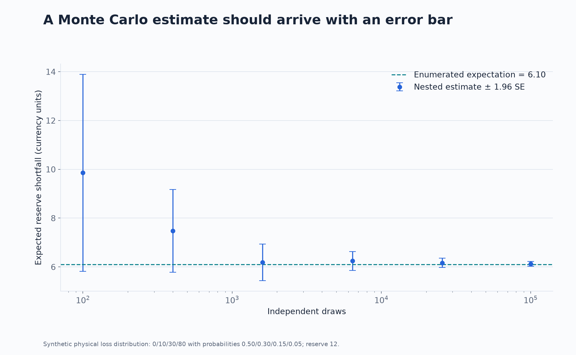
Nested Monte Carlo estimates of a synthetic expected reserve shortfall are displayed with approximate 95 percent intervals around the exact target 6.10

The chart uses one seeded sample and prefixes of increasing length. Estimates at different budgets are therefore dependent. That is fine for illustrating a single run’s evolution, but these points are not independent experiments for estimating coverage or root mean squared error.

What the confidence interval says

For independent draws with finite variance and a sufficiently well-behaved large-sample approximation,

\widehat\theta_N\pm1.96\frac{s_Y}{\sqrt N}

is an approximate 95% confidence interval for the expectation under the chosen model. Its interpretation concerns repeated sampling: the procedure produces intervals containing the fixed model expectation about 95% of the time when the approximation is accurate.

It is not a 95% range for next period’s realised loss. That prediction problem involves the loss distribution itself. It also excludes uncertainty about the probabilities and severity values supplied to the simulation.

Rare events need special attention. If no rare loss appears in a small sample, the resulting sample variance can severely understate uncertainty. Heavy-tailed outcomes can make the normal approximation slow or invalidate a finite-variance formula altogether. A code cell printing an interval does not prove its assumptions hold.

For inference questions and dependence pitfalls, continue to statistics interview questions.

Why four times the work halves the standard error

In this example,

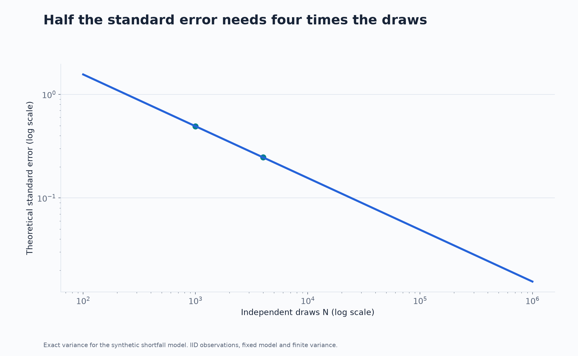
\mathbb E[Y^2]=0.15\times18^2+0.05\times68^2=279.8,

so $\operatorname{Var}(Y)=279.8-6.1^2=242.59$ . The theoretical estimator standard error is $\sqrt{242.59/N}$ .

At 1,000 draws it is about 0.493; at 4,000 draws it is about 0.246. The square-root relationship means that halving standard error requires four times as many independent observations. Reducing it by a factor of ten requires about one hundred times as many.

The theoretical Monte Carlo standard error declines at the inverse square-root rate for independent synthetic shortfalls with fixed finite variance

For a target approximate interval half-width $h$ , an initial budget estimate is

N\approx\frac{1.96^2\operatorname{Var}(Y)}{h^2}.

For $h=0.10$ here, this suggests about 93,194 draws, rounding upward. In a problem with unknown payoff variance, use a separate pilot to plan a production budget. Repeatedly stopping the same experiment whenever an ordinary fixed-sample interval looks narrow enough changes the sampling procedure and may require a sequentially valid method.

More draws are not the only option. Analytic conditioning, control variates, antithetic sampling or importance sampling can reduce variance for suitable targets. Each method changes what counts as an independent observation or how weights must be handled. The option-pricing companion compares two of these methods at equal evaluation budgets.

Four errors that more paths do not all fix

Monte Carlo sampling error is the finite-draw fluctuation around the chosen model’s target. Increasing independent draws addresses it at the usual square-root rate.

Time-discretisation error appears when dynamics or observation rules are approximated. For a continuous-time barrier option, exact stock transitions at daily dates still do not detect every between-date crossing. Refining the time grid or using a compatible bridge correction targets that issue.

Input and model error concern the probability law itself. If the rare-loss probability is wrong, more draws concentrate the estimator around the wrong expectation. Sensitivity scenarios, calibration checks and model comparisons address different questions from sampling precision.

Implementation error includes wrong units, an incorrect payoff, a missing discount factor or a timing mistake. Known identities and small exact examples are more useful than simply increasing the path count.

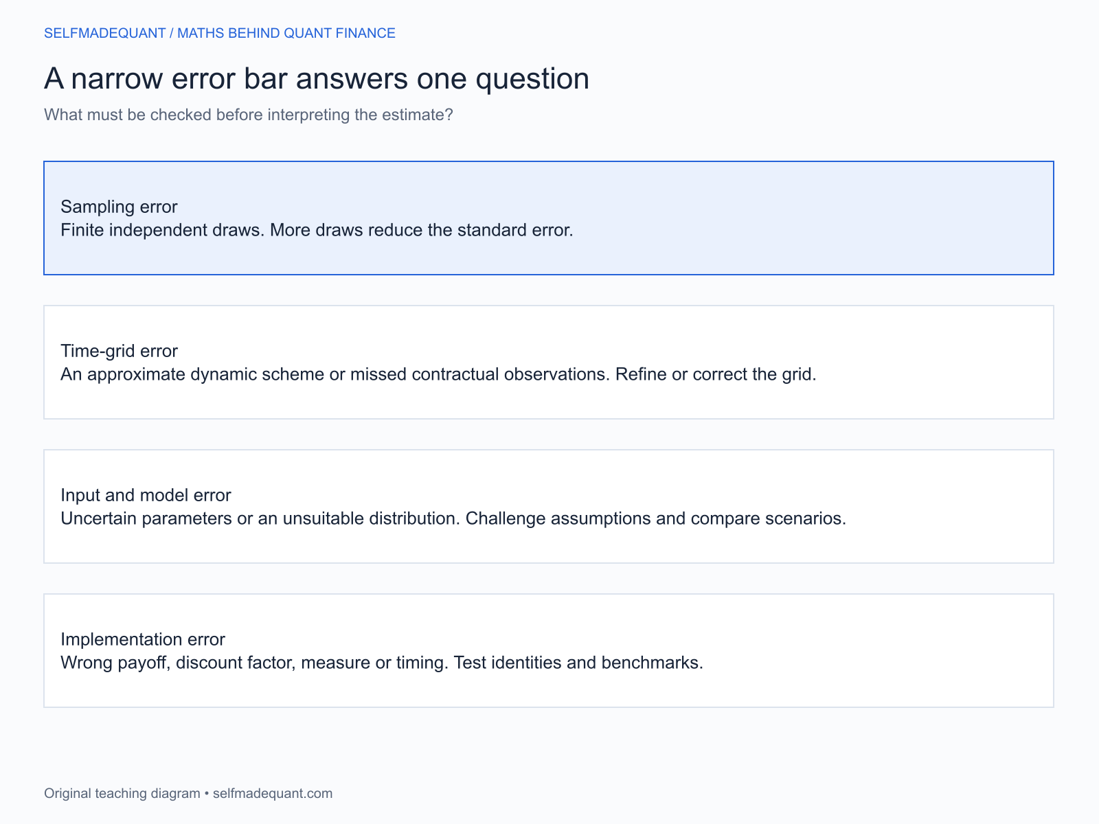
Sampling, time-grid, input and implementation errors require different checks; a small Monte Carlo standard error only addresses finite-draw uncertainty

These categories can coexist. A result can have a tiny standard error and a large systematic bias. Report the interval as conditional on the model and numerical setup that generated it.

Choose the probability measure for the task

Our reserve calculation uses a physical loss distribution supplied directly. It estimates a risk expectation, without claiming to be a traded derivative price.

For a European option in the standard constant-rate framework, the target is instead

V_0=e^{-rT}\mathbb E^{\mathbb Q}[H].

The risk-neutral measure is constrained by the pricing model. Drawing stock paths with an assumed investment return and discounting their option payoffs at the risk-free rate generally does not implement that target.

Similarly, a simulated exposure distribution and a present derivative value need not use the same measure for every layer of the calculation. State the purpose, the measure and the conditioning information before interpreting the output.

Build checks into your first project

Begin with an exactly solvable case, such as the four losses above. Verify that probabilities sum to one, the payoff is nonnegative, and the expectation is no larger than the maximum possible payoff. Check the limiting reserve cases: a reserve of zero estimates expected loss, and a reserve at least 80 makes every shortfall zero.

Next run independent replications with different fixed seeds. Their variation should be broadly consistent with reported standard errors. To estimate interval coverage, count how often independently generated intervals contain the known answer. One interval containing it is only one observation of that experiment.

Finally, vary a meaningful model input separately from the seed. Changing the reserve, loss severity or event probability is a sensitivity analysis; changing only the seed examines numerical sampling variability. Labelling both prevents a chart from mixing distinct sources of uncertainty.

When moving from a toy distribution to actual data, document what was known at the forecast date. A historically estimated input can still contain look-ahead bias if its construction used future information.

Download and take the next step

The stochastic-calculus and Monte Carlo code package includes this reserve example, all numerical charts and the option estimators. It saves a results file and a comparison table so you can inspect numbers as well as figures.

Continue to Monte Carlo option pricing, or repair the simulation foundations with Brownian motion and GBM. For structured learning, the Options Pricing programme connects the model, payoff and numerical method.

Sources and further study

NumPy’s random-generator documentation describes the interface used for sampling. MIT’s Analytics of Finance lecture materials provide further computational-finance context. The reserve distribution and all associated results here are synthetic teaching examples.