One pricing structure, several markets: the Black–Scholes family

Published 10 October 2026Updated 14 October 20265 min readOptions pricing:Part 1 Part 2 Part 3Part 4Part 5 Part 6 Part 7 Part 8

A stock option, a currency option, and an option on a futures contract can look remarkably similar on a pricing screen. They can also use different inputs, discounting conventions, and sources of carry.

Putting spot into a formula that expects a forward is not a small approximation. It changes the economic object being priced. Before changing the volatility model, make sure the underlying, settlement date, discount factor, and forward are aligned.

This article separates market-specific versions of the lognormal formula from models that change the underlying uncertainty. A dividend adjustment and stochastic volatility solve different problems.

We will connect dividend-adjusted Black–Scholes, Garman–Kohlhagen for FX options, Black 76 for futures options, and the Bachelier normal model. The starting point is the Black–Scholes pricing argument; the task here is choosing inputs that describe the actual contract.

The Black–Scholes formula in forward form

For a European call on a terminal underlying level, assume its forward-measure distribution is lognormal with volatility $\sigma$ over $T$ . With deterministic discounting in our examples:

C=D(0,T)\{F_0\Phi(d_1)-K\Phi(d_2)\},

d_1=\frac{\log(F_0/K)+\tfrac12\sigma^2T}{\sigma\sqrt T},\qquad d_2=d_1-\sigma\sqrt T.

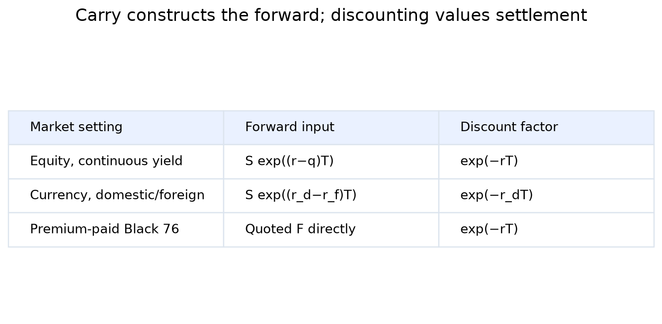
$F_0$ is the forward for the underlying level at the relevant expiry, and $D(0,T)$ discounts the payoff's settlement date. For a spot stock with continuous yield $q$ , $F_0=S_0e^{(r-q)T}$ and $D=e^{-rT}$ . Substituting these recovers the dividend-adjusted BSM formula.

The formula is simpler when we separate carry from uncertainty. Carry determines the forward. Volatility determines the width of the assumed terminal distribution around it. The discount factor translates future money into present money.

That decomposition has limits. Stochastic interest rates and mismatched fixing and payment dates can require a different measure or a convexity adjustment. We do not obtain those adjustments by relabelling $r$ .

Forward and discount conventions in equity currency and futures settings

The table assumes deterministic rates and the stated premium-paid conventions. Contract fixing, settlement and margin details still need checking.

Dividends and equity indices

For a smooth continuous dividend yield, the call is:

C=S_0e^{-qT}\Phi(d_1)-Ke^{-rT}\Phi(d_2).

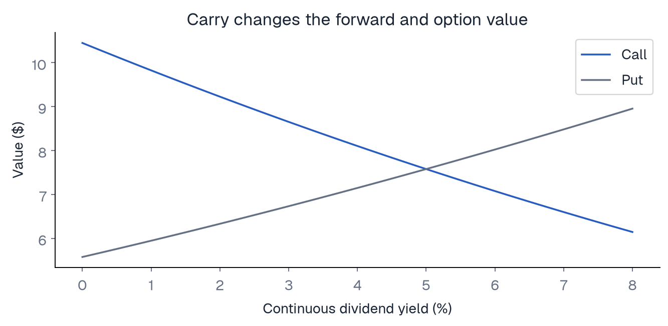
Holding spot and the other inputs fixed, higher $q$ lowers the forward, lowers a European call, and raises a European put. This concerns distributions paid away from the ex-dividend stock. It does not say that all high-dividend stocks have lower option premiums; their volatilities and other inputs may differ.

Synthetic call and put values as dividend yield changes

Only continuous yield changes. Spot, strike, expiry, rates, and volatility are fixed.

Known cash dividends are different. Subtracting their present value from spot and using BSM is a common approximation. It is not automatically an exact solution to a stock process with discrete cash jumps, especially near an ex-dividend date or for American exercise. Model the actual dividend convention when it affects the decision.

Equity index options often use a dividend yield or a directly observed forward. Check whether the contract is cash settled, which fixing determines settlement, and whether the volatility quote corresponds to that same forward.

Garman–Kohlhagen: FX options with two interest rates

Quote $S$ as domestic currency per unit of foreign currency. A domestic investor holding foreign currency can earn the foreign rate $r_f$ . Under standard deterministic-rate assumptions, that acts like a yield:

F_0=S_0e^{(r_d-r_f)T},\qquad C=S_0e^{-r_fT}\Phi(d_1)-Ke^{-r_dT}\Phi(d_2).

This is the Garman–Kohlhagen version. The option value is in domestic currency per foreign currency unit before applying the contract's notional.

Reverse the exchange-rate quote and the interpretation changes. A volatility surface's delta convention may also distinguish spot delta, forward delta, and premium-adjusted delta. A number called “25 delta” is not enough to recreate a strike without knowing that convention.

For a synthetic example, take $S_0=1.10$ domestic per foreign unit, $r_d=4\%$ , $r_f=2\%$ , and $T=1$ . The forward is approximately 1.1222. Inserting 1.10 directly as the forward would discard the rate differential. No volatility adjustment repairs that mismatch reliably.

Futures and Black 76

Black's formula uses a quoted futures or forward level in the appropriate setting:

C=e^{-rT}\{F_0\Phi(d_1)-K\Phi(d_2)\}.

There is no additional $e^{(r-q)T}$ carry step applied to $F_0$ . Doing so carries an already forward-looking price a second time.

For $F_0=K=100$ , $\sigma=20\%$ , $r=5\%$ , and $T=1$ , the premium-paid call is approximately $7.5771$ . Compare that with our spot-stock benchmark carefully: the forward levels differ, so the price difference is not evidence that one formula is wrong.

A futures-style option may use different premium and variation-margin arrangements. Futures and forwards can also differ when rates are stochastic. Contract settlement and the measure behind the formula matter; “Black 76” is not permission to ignore them.

Deterministic time-varying volatility

A lognormal model can allow a deterministic volatility schedule $\sigma(t)$ . For a European terminal payoff, the relevant total variance is:

w(T)=\int_0^T\sigma^2(t)\,dt.

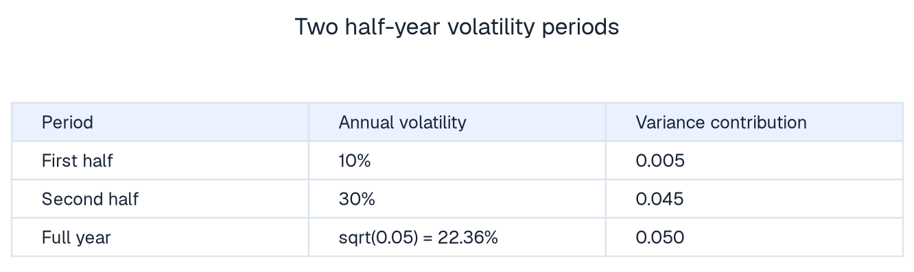
The formula uses $\sqrt{w(T)}$ where constant BSM uses $\sigma\sqrt T$ . If volatility is 10% for half a year and 30% for half a year, total variance is $0.5(0.10)^2+0.5(0.30)^2=0.05$ . The effective annual volatility is $\sqrt{0.05}=22.36\%$ , not the arithmetic average 20%.

This extension can represent a maturity term structure. It still does not generate arbitrary strike-dependent smiles at a fixed expiry. Deterministic volatility changes when uncertainty arrives; stochastic or state-dependent volatility changes how uncertainty depends on the path or state.

Total variance from two half-year volatility periods

Variance contributions add over time. Half a year at 10% and half at 30% produces a 22.36% effective annual volatility.

Bachelier normal pricing and displaced diffusion

A lognormal forward stays positive. That can be unsuitable for markets where the quoted underlying can be negative. The Bachelier model assumes normally distributed forward changes and uses a normal volatility $\sigma_N$ with price units per square-root year:

C=D\{(F_0-K)\Phi(d)+\sigma_N\sqrt T\varphi(d)\},\qquad d=\frac{F_0-K}{\sigma_N\sqrt T}.

Normal volatility is not interchangeable with percentage lognormal volatility. At the money, one compares prices or uses a stated approximate conversion; one does not copy the same numeric input between formulas.

A displaced diffusion assumes $F+a$ is lognormal for a shift $a$ . Then shifted forward and shifted strike enter the lognormal formula, provided both are positive. The shift changes distributional support and smile behavior. It is a modeling choice, not merely an extra dividend yield.

A practical input checklist

Write down the underlying quotation, option exercise rule, payoff currency, expiry and settlement dates, forward or carry convention, discount curve, and volatility units. Confirm that all inputs describe the same contract. Then validate put–call parity in that convention.

These details are the bridge between classroom formulas and usable implementations. In Monte Carlo option pricing, we hold the model fixed and change the solver, reproducing the same European price while making sampling error visible.

Continue learning

Work through futures options and Black's model and the continuous-dividend PDE derivation.

Sources

Black, “The pricing of commodity contracts” (1976); Garman and Kohlhagen, “Foreign currency option values” (1983). The normal and shifted-lognormal formulas are mathematical comparisons, not recommendations for a particular market.