Itô’s lemma explained: intuition, derivation and worked examples

Published 15 October 20265 min readThe maths behind quant finance:Part 1 Part 2Part 3Part 4 Part 5 Part 6

Itô’s lemma is the chain rule for a smooth function of an Itô diffusion. Besides the ordinary time and first-derivative terms, it includes half the diffusion variance multiplied by the function’s second derivative.

That extra term explains why a geometric Brownian stock model with proportional drift $\mu$ has expected log growth $\mu-\sigma^2/2$ . It also appears in the Black–Scholes equation. Missing it changes both simulated distributions and derivative prices.

We will derive the correction’s intuition from squared increments, state the formula precisely enough to use, then work through three examples. Basic derivatives and Brownian motion are the prerequisites. The derivation below motivates the theorem; it is not a replacement for the stochastic-integral limit arguments in a full proof.

The formula, with each term identified

Suppose

dX_t=a(t,X_t)\,dt+b(t,X_t)\,dW_t

is a well-defined continuous Itô process with the required local integrability, and $f(t,x)$ is once continuously differentiable in time and twice continuously differentiable in its state variable. Then

df(t,X_t)=\left(f_t+a f_x+\tfrac12b^2f_{xx}\right)dt+b f_x\,dW_t.

All derivatives and coefficients on the right are evaluated at $(t,X_t)$ . The equivalent integral statement is

\begin{aligned} f(t,X_t)-f(0,X_0) ={}&\int_0^t\left(f_t+a f_x+\tfrac12b^2f_{xx}\right)(u,X_u)\,du\\ &+\int_0^t(b f_x)(u,X_u)\,dW_u. \end{aligned}

The first integral is an ordinary time integral. The second is an Itô stochastic integral. Its construction uses integrands that do not look into future increments. The familiar differential notation is shorthand for this integral relationship.

Ingredient	Meaning	What it contributes
Time derivative	The function changes even if the state is held fixed	Time drift
First state derivative	Local sensitivity to a change in the state	State drift and random exposure
Second state derivative	Curvature of the function	Additional drift from accumulated squared noise

For a linear function of the state, the curvature is zero and the correction vanishes. For nonlinear functions, it generally does not.

Why the ordinary chain rule misses a term

Over a small interval, write $\Delta X\approx a\Delta t+b\Delta W$ . A second-order Taylor expansion suggests

\Delta f\approx f_t\Delta t+f_x\Delta X+\tfrac12 f_{xx}(\Delta X)^2.

The squared state increment expands as

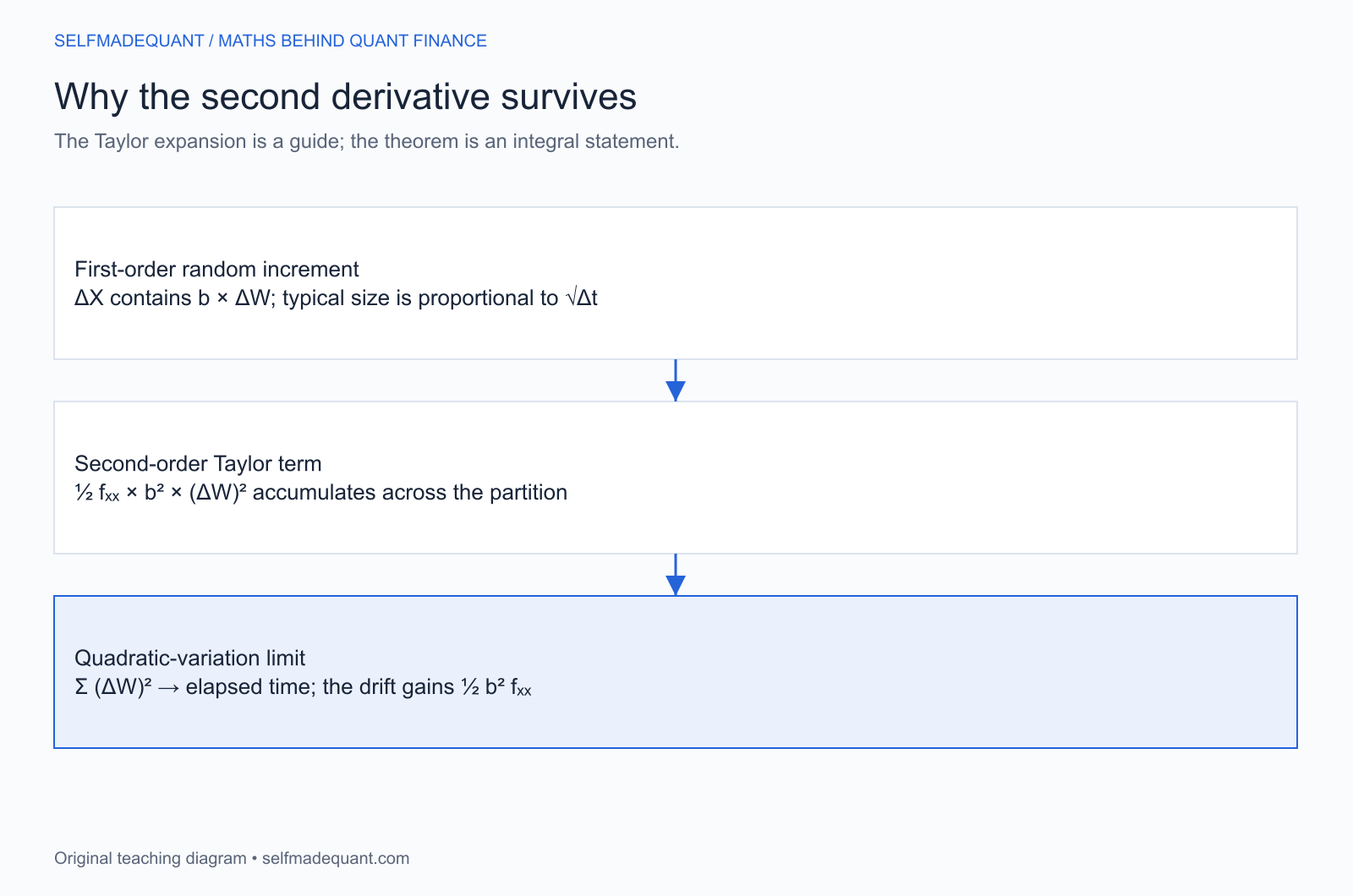
(\Delta X)^2\approx a^2(\Delta t)^2+2ab\Delta t\Delta W+b^2(\Delta W)^2.

Brownian increments have typical scale $\sqrt{\Delta t}$ . The final term therefore has the same accumulated order as elapsed time. On finer partitions, the time-square and mixed terms vanish under the theorem’s conditions, while squared Brownian increments accumulate into quadratic variation.

That leaves $\tfrac12b^2f_{xx}dt$ . The shorthand rules $dt^2=0$ , $dt\,dW=0$ and $(dW)^2=dt$ help remember the calculation, but the actual justification is convergence of sums. A finite squared increment is still random.

The Itô correction arises because the second-order Taylor term contains squared Brownian increments whose sum converges to elapsed time

There is also a timing choice. An Itô sum evaluates the integrand at the left endpoint, before the next increment is known. A Stratonovich integral uses a different limiting convention and a different chain rule. Changing convention without converting the drift changes the mathematical model.

Example 1: the square of Brownian motion

Let $X_t=W_t$ and $f(x)=x^2$ . Here $a=0$ , $b=1$ , $f_x=2x$ , $f_{xx}=2$ and $f_t=0$ . Substitution gives

d(W_t^2)=dt+2W_t\,dW_t.

Starting from $W_0=0$ ,

W_t^2=t+2\int_0^t W_u\,dW_u.

The stochastic integral has mean zero on a finite horizon because its integrand satisfies the needed square-integrability condition. Therefore $\mathbb E[W_t^2]=t$ , agreeing with the Brownian variance.

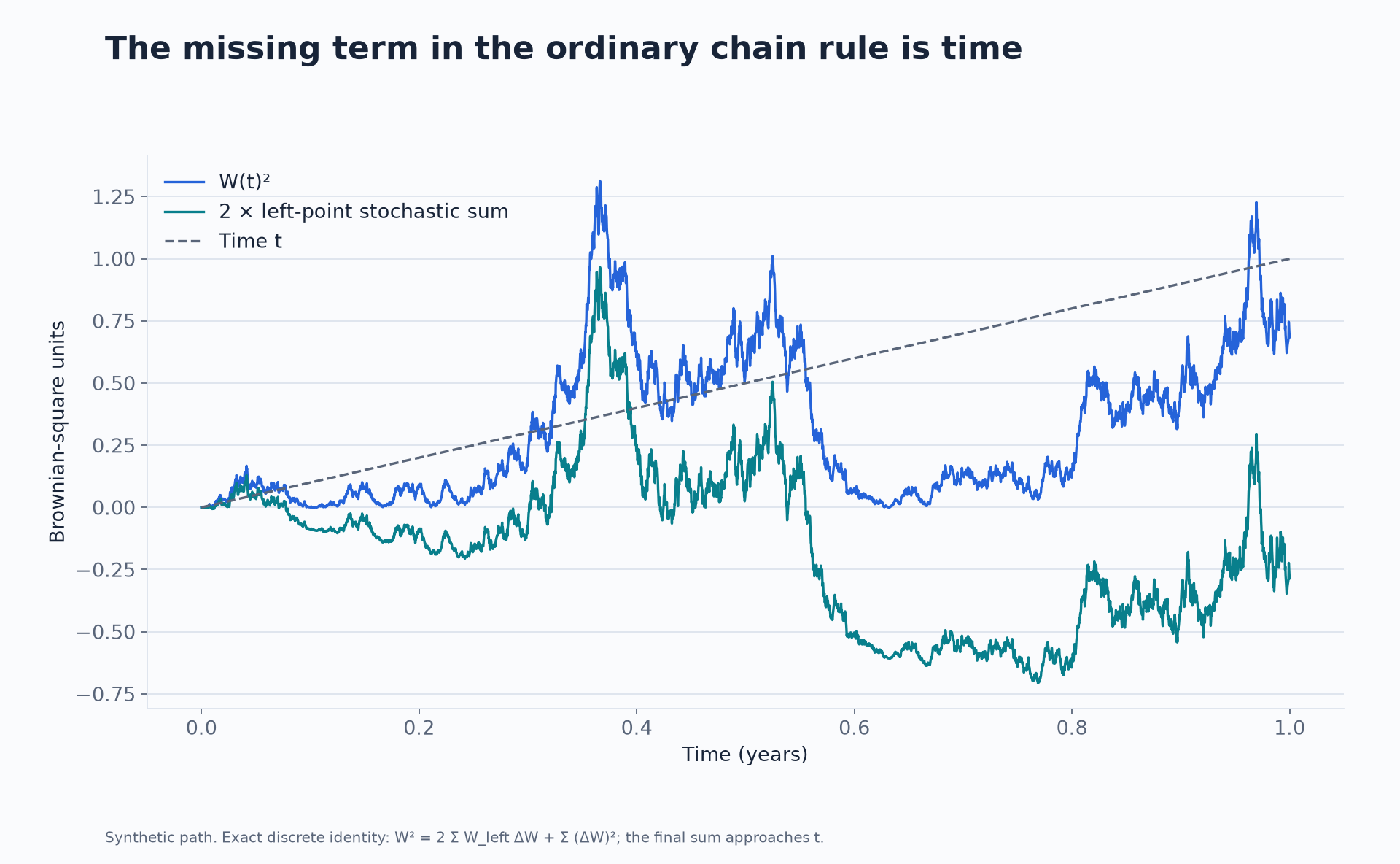
There is an exact discrete identity behind the picture:

W_{t_{i+1}}^2-W_{t_i}^2 =2W_{t_i}\Delta W_i+(\Delta W_i)^2.

Summing telescopes. The left-point sum approaches the stochastic integral, while the sum of squares approaches $t$ . The finite-grid identity is exact even though replacing the sum of squares by time is a limiting step.

import numpy as np

rng = np.random.default_rng(20261015)
increments = rng.normal(0.0, np.sqrt(1 / 4096), 4096)
w = np.r_[0.0, np.cumsum(increments)]
left_sum = np.sum(w[:-1] * increments)
quadratic_sum = np.sum(increments**2)
residual = w[-1]**2 - 2 * left_sum - quadratic_sum
print(f"quadratic sum={quadratic_sum:.6f}")
print(f"discrete identity residual={abs(residual):.2e}")
# quadratic sum=0.970260
# discrete identity residual=5.55e-16

The residual checks floating-point arithmetic in a discrete identity. It is not an estimate of the error in a general Itô theorem. The quadratic sum’s distance from 1 is the finite-partition fluctuation relevant to this example.

Brownian square equals twice the left-point stochastic sum plus quadratic variation; the accumulating correction is approximately time on a fine grid

The connection to martingales is immediate:

W_t^2-t

is a martingale, whereas

W_t^2

has positive expected drift.

Example 2: log of a geometric Brownian stock price

Assume a strictly positive stock process obeys

dS_t=\mu S_t\,dt+\sigma S_t\,dW_t

with constant coefficients. For $f(s)=\log s$ on $s>0$ ,

f_s=1/s,\qquad f_{ss}=-1/s^2.

Using $a=\mu S$ and $b=\sigma S$ yields

d\log S_t=(\mu-\tfrac12\sigma^2)dt+\sigma\,dW_t.

Integrate and exponentiate:

S_t=S_0\exp\left((\mu-\tfrac12\sigma^2)t+\sigma W_t\right).

If $\mu=8\%$ per year and $\sigma=30\%$ per square-root year, the correction is $0.5\times0.3^2=0.045$ per year. Expected log growth is $0.08-0.045=0.035$ , or 3.5% per year.

That does not mean the expected stock price grows at 3.5%. Exponentiation is nonlinear. The Gaussian exponential moment restores the expected price growth to

e^{\mu t}

. The GBM article separates the mean, median and expected log return numerically.

The domain matters: log is undefined at nonpositive prices. Exact GBM stays positive from a positive starting value, but an Euler approximation can produce a negative step. Taking a logarithm after such a step does not fix the discretisation.

Example 3: an exponential martingale

Take $f(t,w)=\exp(\sigma w-\sigma^2t/2)$ . Its derivatives are

f_t=-\tfrac12\sigma^2f,\qquad f_w=\sigma f,\qquad f_{ww}=\sigma^2f.

For $X=W$ , the two drift terms cancel:

df(t,W_t)=\sigma f(t,W_t)\,dW_t.

This identifies the local-martingale form. For this constant-coefficient example, the Gaussian exponential moment additionally proves the true martingale property on finite horizons. That extra check matters: zero drift in a formal differential does not establish the needed integrability for every model.

The same exponential structure appears in a discounted, non-dividend-paying GBM stock under the risk-neutral measure. Risk-neutral pricing explains why the drift becomes the risk-free rate for this pricing calculation.

How this enters the Black–Scholes equation

Let $V(t,S)$ be a sufficiently smooth option value in the interior of its time domain. Itô’s lemma gives

dV=\left(V_t+\mu S V_S+\tfrac12\sigma^2S^2V_{SS}\right)dt+\sigma S V_S\,dW.

A delta hedge holds $V_S$ shares against the option. Within the frictionless continuous-trading replication argument, the stock exposure cancels the random term. No arbitrage requires the remaining locally riskless position to earn the risk-free rate. For a stock without dividends,

V_t+\tfrac12\sigma^2S^2V_{SS}+rS V_S-rV=0.

The physical drift $\mu$ disappears from this replication equation. Itô’s lemma supplies the option dynamics; self-financing replication and no arbitrage supply the pricing restriction. The calculus alone does not establish a market price.

At maturity a call payoff has a kink at the strike and is not twice differentiable there. The familiar pricing derivation uses the smooth pre-maturity value function, with the payoff imposed as a terminal condition. You cannot apply the elementary smooth version directly at every point of a nonsmooth payoff. Generalisations such as Itô–Tanaka handle particular nonsmooth functions with additional terms.

For the full financial argument and assumptions, continue to Black–Scholes explained.

A repeatable method for new functions

First identify the state dynamics and the probability measure. Then calculate the three derivatives of the transformed function. Substitute the actual diffusion coefficient into $b^2$ , including any state factors. Finally collect the drift and diffusion separately and check a known implication.

For $f(S)=S^2$ under GBM, this gives

d(S_t^2)=(2\mu+\sigma^2)S_t^2dt+2\sigma S_t^2dW_t.

The positive $\sigma^2$ term is consistent with increasing second moments. Leaving it out would understate the model’s expected square and variance.

For a deterministic state with $b=0$ , the formula reduces to the ordinary chain rule. For a linear function with $f_{xx}=0$ , there is no curvature correction. These boundary checks catch many sign and coefficient mistakes before simulation does.

Download and continue

The stochastic-calculus code package includes the discrete identity experiment, GBM figures and option estimators. It uses synthetic inputs and records its seeds and outputs.

Study the Options Pricing programme, starting with Brownian motion and Itô’s lemma, then market models and risk-neutral valuation. The next article solves and simulates geometric Brownian motion.

Sources and further study

MIT’s Itô calculus lecture provides a university video treatment. For a more recent lecture, watch MIT’s stochastic calculus introduction on YouTube. MIT’s 2024 finance mathematics course, Week 14 offers further stochastic-calculus materials. The derivations and numerical examples here are presented independently.