Risk-neutral pricing explained: a two-state replication example

Published 15 October 20266 min readThe maths behind quant finance:Part 1 Part 2 Part 3 Part 4Part 5Part 6

Risk-neutral pricing values a payoff by taking its expectation under pricing probabilities and discounting at the risk-free rate. Those probabilities are chosen to make traded asset prices consistent with no arbitrage. They are not automatically forecasts of how often market outcomes will occur.

The cleanest way to see why this works is to price the same call twice: first by replicating its payoff with a stock and a bond, then by constructing probabilities that give the identical answer. No stochastic calculus is required.

Our example assumes two possible future stock values, no dividends or transaction costs, and the ability to buy, sell, borrow and lend at the stated prices. These assumptions let us isolate the pricing argument. We will relax the interpretation afterward.

The entire market fits in a table

Today’s stock price is 100. One period from now it will be either 120 or 80. A risk-free investment grows by a factor of 1.05 over the period. A European call has strike 100 and pays 20 in the up state and zero in the down state.

Instrument	Today	Up state	Down state
One share	100	120	80
One unit invested in the bank	1	1.05	1.05
Call, strike 100	To calculate	20	0

The 1.05 is a one-period gross growth factor. We are not treating it as $e^{0.05}$ ; that would be a different interest-rate convention. If the period were one year and the rate were continuously compounded, the corresponding rate here would be $\log(1.05)$ .

We have not supplied the actual chance of an up move. Surprisingly, we can still price the call in this complete two-state model.

Replicate the payoff with a stock and a bond

Hold $\Delta$ shares and put $B_0$ in the bank. A negative bank position means borrowing. Matching the call in both states requires

120\Delta+1.05B_0=20,\qquad 80\Delta+1.05B_0=0.

Subtract the equations:

40\Delta=20\quad\Rightarrow\quad\Delta=0.5.

Substitute into the down state:

40+1.05B_0=0\quad\Rightarrow\quad B_0=-40/1.05.

The hedge buys half a share and borrows 38.095238. Its initial cost is

C_0=100\times0.5-\frac{40}{1.05}=11.904762.

In the up state, the half-share is worth 60 and the debt is 40, leaving 20. In the down state, it is worth 40 and the debt is 40, leaving zero. Every modelled state matches the call exactly.

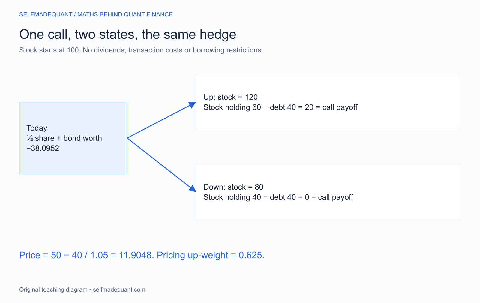
Half a share financed by borrowing 38.0952 today reproduces the call payoff in both future states, giving a price of 11.9048

This is why the initial prices must agree. If the call costs more than the replicating portfolio, sell the call and buy the portfolio. Their future cash flows offset, leaving an initial surplus. If it costs less, reverse the trade. Under the market assumptions, either discrepancy would create an arbitrage.

The conclusion comes from matching state-by-state cash flows, rather than guessing an investor’s attitude toward risk.

Derive the risk-neutral probability

Let $p^*$ be an up-state pricing probability. Require the stock’s discounted expected value to equal its current price:

100=\frac{120p^*+80(1-p^*)}{1.05}.

Solving gives

p^*=\frac{105-80}{120-80}=0.625.

Now price the call by the same rule:

C_0=\frac{0.625\times20+0.375\times0}{1.05}=11.904762.

It matches replication exactly. The probabilities are a convenient representation of the no-arbitrage pricing rule already established by the hedge.

In the familiar notation $S_u=S_0u$ , $S_d=S_0d$ and bank factor $R$ ,

p^*=\frac{R-d}{u-d},\qquad V_0=\frac{p^*V_u+(1-p^*)V_d}{R}.

Here $u=1.2$ , $d=0.8$ and $R=1.05$ . We use $p^*$ rather than $q$ for the pricing probability because $q$ often denotes a dividend yield in continuous-time option models.

s0, up, down, bank = 100.0, 120.0, 80.0, 1.05
call_up, call_down = 20.0, 0.0
delta = (call_up - call_down) / (up - down)
bond = (call_down - delta * down) / bank
p_star = (bank * s0 - down) / (up - down)
replication = delta * s0 + bond
expectation = (p_star * call_up + (1 - p_star) * call_down) / bank
print(f"delta={delta:.3f}, bond={bond:.6f}, p*={p_star:.3f}")
print(f"replication={replication:.6f}, expectation={expectation:.6f}")
# delta=0.500, bond=-38.095238, p*=0.625
# replication=11.904762, expectation=11.904762

Why the probability must lie between zero and one

The strict no-arbitrage condition in this nondegenerate model is

S_d<RS_0<S_u,

or equivalently $d<R<u$ . It ensures $0<p^*<1$ when both states are possible under the physical model.

If $RS_0<S_d$ , borrowing to buy the stock produces a positive net payoff even in the lower stock state. If $RS_0>S_u$ , shorting the stock and investing the proceeds produces a positive net payoff even in the higher state. Equality at an endpoint also gives an arbitrage with a positive payoff in one possible state and zero in the other under these assumptions.

An out-of-range “probability” is therefore a diagnostic of inconsistent input prices, rather than a number to clip into the interval. Clipping would conceal the violation and alter the pricing rule.

In this two-state market, the stock and bond span both state payoffs. The pricing probability is unique. In incomplete markets with risks that cannot all be replicated, no arbitrage alone need not determine a unique pricing measure or a unique price for every claim.

Physical probabilities answer a different question

Suppose you believe the actual up probability is 70%. The physical expected call payoff is $0.7\times20=14$ . Discounting it at the bank factor produces $14/1.05=13.333333$ , which differs from the replication price.

That calculation has discounted a risky expected payoff as if the bank rate were its appropriate risk-adjusted discount rate. It does not override the state-by-state hedge available for 11.904762.

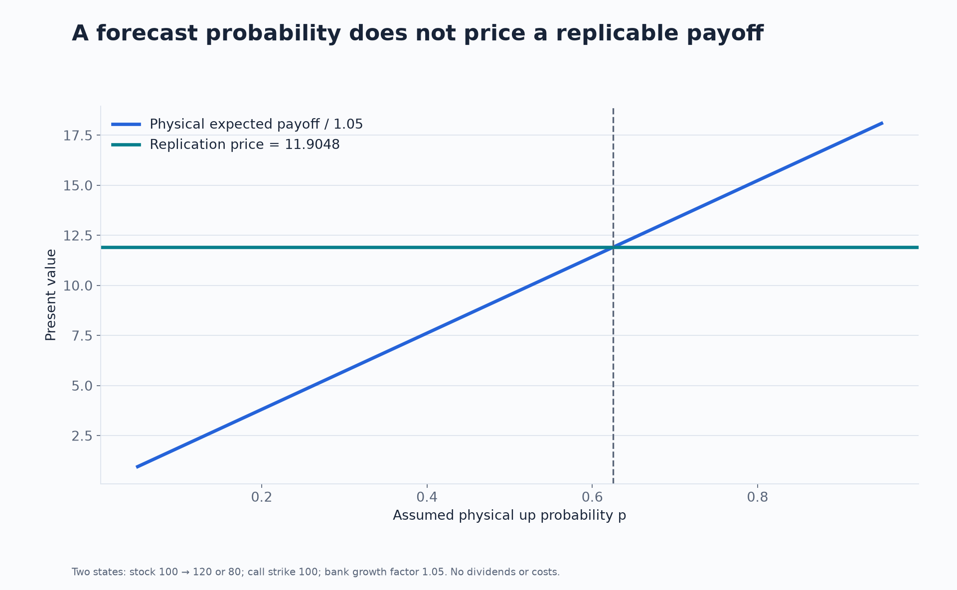
Discounting a physical expected call payoff at the bank rate gives different values as the forecast probability changes, while the replication price stays fixed

The physical expected stock return under the 70% forecast is $0.7\times20\%+0.3\times(-20\%)=8\%$ , above the bank’s 5%. The pricing probability gives expected stock growth of 5%. These are two distinct probability descriptions serving different purposes.

“Risk-neutral” does not require actual investors to be indifferent to risk. Their preferences and beliefs help determine traded prices. Once those prices are given, replication constrains the derivative price in this model. The pricing measure encodes that constraint.

For a portfolio risk forecast, a physical distribution may be the relevant object. For a replicable derivative price, the pricing measure is the relevant object. Some practical systems use both, with physical scenarios for future exposures and risk-neutral valuation inside each scenario; the two layers must be labelled.

State prices reveal the same structure

Define the present prices of one unit paid only in a particular state:

\pi_u=\frac{p^*}{R},\qquad \pi_d=\frac{1-p^*}{R}.

Then $V_0=\pi_uV_u+\pi_dV_d$ . The state prices are positive and sum to $1/R$ , because a unit paid in either state is a risk-free future unit. Multiplying the state prices by $R$ turns them into probabilities that sum to one.

This offers a useful interpretation: risk-neutral probabilities are normalised pricing weights. Their connection to today’s traded prices is essential. Arbitrary probabilities that happen to sum to one do not establish a valid pricing model.

Connect the tree to martingales and continuous time

At each node of a multi-period tree, the same one-step rule makes the bank-discounted stock a martingale under the pricing measure. Work backward through the tree to value a European payoff. For American exercise, compare immediate exercise with continuation at each permitted date.

The binomial option-pricing article develops that recursion. A larger tree adds dates and states; it does not remove the need to specify dividends, rates and exercise rules correctly.

In the constant-rate, constant-volatility GBM model, the risk-neutral drift is

r-q

for a stock paying continuous dividend yield

q

. A European payoff

H

is valued as

V_0=e^{-rT}\mathbb E^{\mathbb Q}[H].

The rate $r$ here is continuously compounded, unlike the simple one-period factor used above. With stochastic rates, discounting belongs inside the expectation as the appropriate random discount factor, subject to the pricing framework and numeraire choice.

The Monte Carlo option-pricing guide estimates this expectation from simulated risk-neutral outcomes. Increasing its path count cannot correct the use of a physical drift in place of a pricing drift.

Check your understanding

If the physical up probability changes from 70% to 60% while the stock, bond and state prices in the example are held fixed, the replication price stays 11.904762. The physical expected payoff changes, but the hedge has not changed.

If the up-state stock price changes, the hedge ratio and pricing probability generally change. That is an alteration to the market model itself. If a trading restriction prevents borrowing or shorting, the unrestricted replication and arbitrage argument may no longer be implementable.

These distinctions explain both the power and the scope of the result: one price follows from a particular set of tradable instruments and assumptions.

Download and continue studying

The series code package includes this hedge calculation and the continuous-model simulations. Use it to change one input at a time and check whether replication and pricing expectation still agree.

For a complete sequence, study Options Pricing, starting with market models and risk-neutral valuation and the binomial model.

Sources and further study

MIT’s risk-neutral valuation lecture develops the continuous-time connection. The two-state example and its code are original calculations under the assumptions stated above.