Beyond Black–Scholes: what changes when volatility becomes a state?

Published 10 October 2026Updated 14 October 20264 min readOptions pricing:Part 1 Part 2 Part 3 Part 4 Part 5Part 6Part 7 Part 8

Your BSM implementation reproduces the benchmark to ten decimal places. Yet a single volatility input cannot reproduce an observed option surface across strikes.

The solver may be correct. The model may be too restrictive.

A constant-volatility diffusion assigns one terminal distribution to each maturity. Market prices can imply different BSM volatilities at different strikes. We can use those implied volatilities as a quoting surface, but pricing a path-dependent claim or modeling future smile movement requires additional assumptions.

The next choices include Dupire local volatility, Heston stochastic volatility, and Merton jump-diffusion. Each changes a different part of the economic model. More parameters do not automatically produce more reliable hedges. Keep the Black–Scholes assumptions and implied-volatility definition beside these extensions so the comparison stays explicit.

Implied volatility and the volatility smile

Given a European option price, implied volatility is the scalar that reproduces it in BSM. Using a different scalar for every strike can match many individual prices. That operation does not by itself define a single coherent process for the underlying through time.

For a barrier option, the path to expiry matters. Two models can agree on a set of terminal vanilla prices while disagreeing on barrier crossings. A good fit to today's smile cannot settle that disagreement.

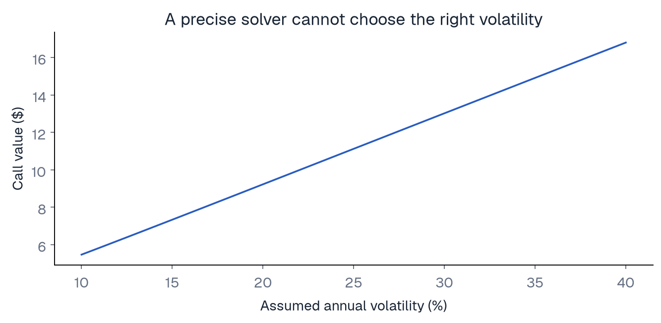
Call values as the assumed constant volatility changes

This synthetic sensitivity plot changes a BSM input. It is not a market smile or a calibrated comparison of richer models.

Consider our $100$ spot, $100$ strike, one-year call. Changing volatility from 20% to 25% moves its model price by far more than the small solver errors we will report in the lab. Numerical precision helps only after we have made the appropriate modeling choices.

Dupire local volatility: a function of spot and time

Under a local-volatility model:

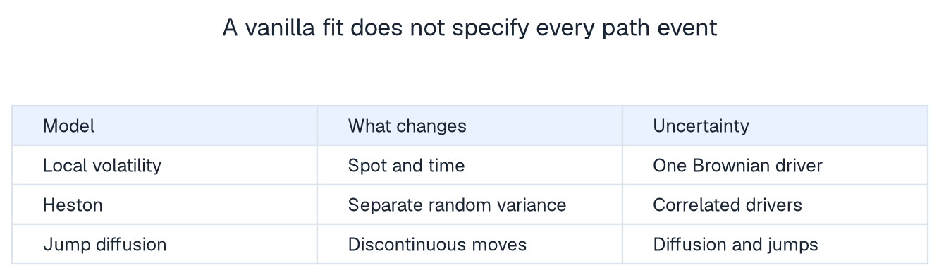
dS_t=(r-q)S_tdt+\sigma_{\mathrm{loc}}(S_t,t)S_tdW_t^{\mathbb Q}.

The function is deterministic, but the realized volatility along a path varies because spot changes. There is still one Brownian driver. With sufficient regularity and ideal arbitrage-free vanilla data, a local-volatility surface can be constructed to match a continuum of European prices.

For constant rates and yield, Dupire's relation expresses local variance in terms of the call surface $C(K,T)$ :

\sigma_{\mathrm{loc}}^2(K,T)= \frac{C_T+(r-q)KC_K+qC}{\tfrac12K^2C_{KK}}.

The derivatives reveal an important practical issue. Market quotes are discrete and noisy. Differentiating them, especially twice in strike, can magnify noise. Interpolation must preserve appropriate no-arbitrage conditions, and tiny denominators in the wings can make the reconstruction unstable.

Matching today's European prices is a calibration property. It is not proof that the future dynamics of the smile, or the hedge of an exotic, are correctly captured. We need tests related to the contract's actual exposure.

Comparison of local volatility Heston and jump diffusion

These models change different assumptions about the path. A common vanilla fit does not make their path-dependent valuations identical.

The Heston stochastic-volatility model

Heston uses stochastic variance $v_t$ :

dS_t=(r-q)S_tdt+\sqrt{v_t}S_tdW_t^S,

dv_t=\kappa(\theta-v_t)dt+\xi\sqrt{v_t}dW_t^v,\qquad d\langle W^S,W^v\rangle_t=\rho\,dt.

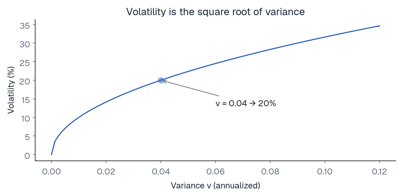
Initial variance $v_0$ sets today's state. $\theta$ is the long-run variance level under the pricing measure. $\kappa$ controls reversion speed. $\xi$ is volatility of variance, and $\rho$ couples stock and variance shocks. Variance is the square of volatility: $v_0=0.04$ corresponds to volatility 20%.

Negative correlation can produce equity-style asymmetry: down moves tend to coincide with higher variance. It does not mean every parameter set generates the right observed skew. Calibration, maturity, and the other parameters matter together.

The Feller condition $2\kappa\theta\ge\xi^2$ is associated with strict positivity of the continuous-time variance process when starting positive. Violating it does not make Heston automatically meaningless; the boundary becomes attainable. A naive Euler simulation can generate negative variance even when the continuous process remains nonnegative. The numerical scheme needs separate care.

A stock and bank alone generally do not span the extra variance risk. Risk-neutral parameters incorporate a choice about its pricing. Do not copy estimates from historical variance dynamics into a pricing model without considering this distinction.

Heston's characteristic function is tractable. That creates a bridge to Fourier option pricing. The model's price is often called semi-analytic because evaluation still involves numerical integration; “closed form” does not always mean elementary arithmetic and normal CDF calls.

Conversion between variance and volatility

The highlighted point is v=0.04, corresponding to 20% volatility. A variance input of 0.20 would imply a very different volatility.

Merton jump-diffusion and the limits of delta hedging

Merton's jump-diffusion adds sudden proportional jumps. One risk-neutral representation is:

\frac{dS_t}{S_{t-}}=(r-q-\lambda k_J)dt+\sigma dW_t+(J-1)dN_t,

where $N_t$ is a Poisson process of intensity $\lambda$ , $J$ is a positive jump multiplier, and $k_J=\mathbb E[J-1]$ . The compensation term $-\lambda k_J$ preserves the desired expected carry.

A continuous delta hedge cannot guarantee cancellation of a finite jump. The option changes nonlinearly across the jump while the stock hedge is fixed immediately before it. More frequent scheduled rebalancing cannot eliminate every surprise discontinuity.

A risk-neutral jump distribution is a pricing assumption, not merely the observed historical distribution. Richer tail behavior may improve a vanilla fit, but it adds parameters and potential instability. It also changes the meaning of hedging residuals.

Calibration is an inverse problem

A forward problem maps parameters to prices. Calibration runs backwards: choose parameters that fit selected prices. Specify the quote timestamps, discount and forward curves, weighting, parameter constraints, and objective. Price-error weighting and implied-volatility-error weighting need not produce the same fit.

Several parameter combinations can explain similar prices. Thinly quoted wings provide weak information. A lower fitting error can coexist with unstable parameters, poor extrapolation, and expensive hedging. Hold out maturities or strikes when assessing fit, and test stability as quotes change.

Choose the next model by the risk you need to represent. A European vanilla quote, a continuously monitored barrier, and a long-dated volatility-sensitive contract do not place identical demands on the model. Today's fit, numerical stability, computational budget, and hedge behavior all matter.

Try it

Write down one feature that a deterministic term-volatility model changes, one that local volatility changes, and one that Heston changes. Then identify a contract whose value depends on the path rather than only the final stock price. Explain why matching European prices alone does not determine its value.

Continue learning

Study stochastic volatility and Heston and simulating SDEs.

Sources

Dupire, “Pricing with a Smile” (1994); Heston, “A Closed-Form Solution for Options with Stochastic Volatility” (1993); Merton, “Option pricing when underlying stock returns are discontinuous” (1976). MathWorks' Heston numerical-integration documentation illustrates the distinction between the model and its integration method.