Binomial option pricing: build the hedge, then work backwards

A pricing formula returns one number. A tree shows the decisions that produce it.

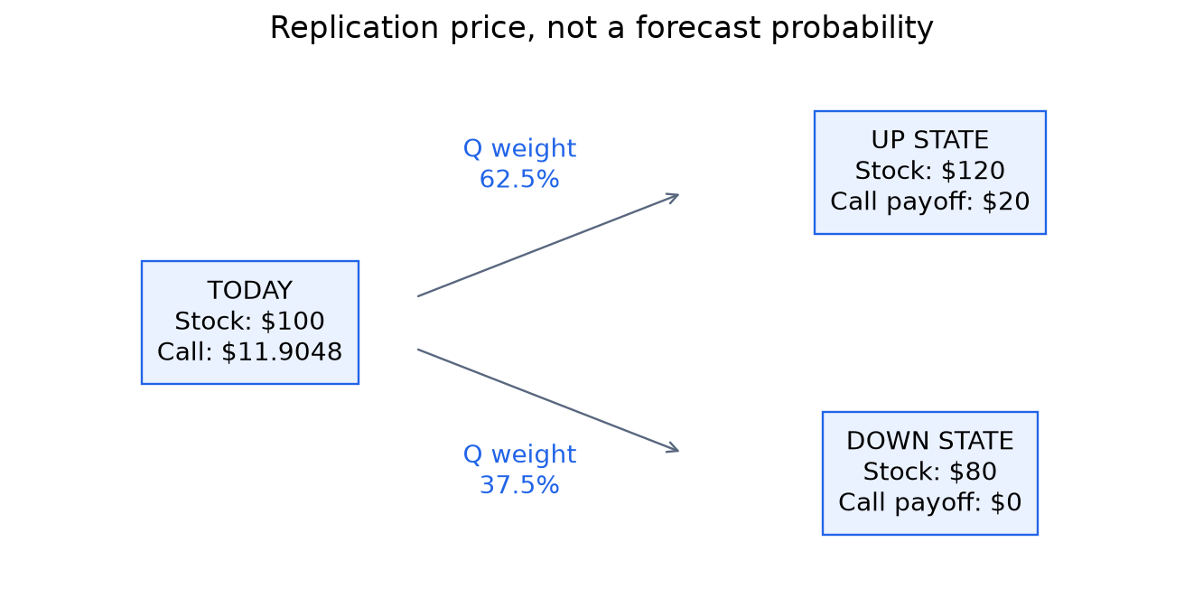
Suppose a stock is at $100 and can move to $120 or $80 in a year. A $100-strike call pays $20 or zero. We can reproduce those payoffs with half a share and borrowing. Its price follows from that hedge, not from guessing which terminal outcome is more likely.

Now repeat the idea over many short intervals. At each node, price the next pair of possible outcomes. Work backwards to today. This is the binomial method, and it becomes especially useful when a contract includes an early-exercise decision.

Replication and the risk-neutral probability at one node

Let a stock be worth $S$ at a node. Next period it is $Su$ or $Sd$, with $u>d$. Assume no dividends in this first derivation and let the bank grow by $R$.

If the option's next values are $V_u$ and $V_d$, the hedge solves:

Therefore:

The condition $d<R<u$ keeps $p$ between zero and one. It also prevents the stock or bank from dominating the other asset in every state. If your implementation produces $p=1.2$, clipping it to one changes the model and hides the problem. Revisit the step size and parameters.

For $u=1.2$, $d=0.8$, and $R=1.05$, the call price is $11.9048$. The up-state pricing probability is 0.625. A historical estimate of 0.60 is irrelevant to this complete two-state replication calculation.

The Cox–Ross–Rubinstein binomial tree

The Cox–Ross–Rubinstein construction uses $N$ intervals of size $\Delta t=T/N$:

Here $q$ is a continuous dividend yield. The $u,d$ steps describe the ex-dividend stock; $r-q$ sets its risk-neutral carry. These equations are a numerical construction aimed at the diffusion limit. For very coarse steps or extreme carry, the probability may be invalid.

The identity $ud=1$ makes the tree recombine: up then down reaches the same price as down then up. At time step $n$, the distinct prices are:

There are $n+1$ nodes at that time, rather than $2^n$ separate histories. Recombination makes vanilla pricing manageable. A payoff that depends on the entire running average cannot generally be valued using only this stock-price node: paths reaching the same stock price can have different averages.

At expiry, assign the contract's payoff to every node. For a European call, $V_{N,j}=\max(S_{N,j}-K,0)$. Then repeat:

Keep the indexing explicit. In this convention $j$ counts up moves. The upper child receives probability $p$. Reversing the weights is an easy bug that can produce plausible-looking prices.

American option pricing and early exercise

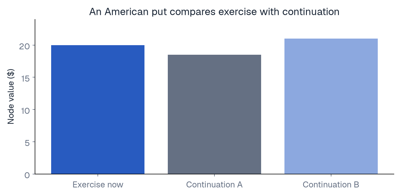
At a node an American put can be exercised for $K-S$. Its owner compares immediate exercise with continuation:

Suppose a put can receive $20 immediately, while its discounted continuation value is $18.50. The node value is $20$. Exercising exchanges remaining optionality for cash now. Positive rates can make receiving the strike earlier valuable.

That does not mean every in-the-money put should be exercised. If continuation is $21$, waiting is worth more than the immediate $20. Moneyness and optimal exercise answer different questions.

For a non-dividend-paying stock under the usual frictionless assumptions and nonnegative rates, early exercise of an American call is not optimal. Exercise gives up remaining protection and requires paying the strike sooner. Dividends can change that conclusion. A continuous yield is a smooth approximation; an actual discrete ex-dividend date may require a tree specifically designed for cash dividends.

The European and American prices must be computed with the same parameters and grid if we want to interpret their difference as the numerical early-exercise premium. Our lab checks that the American put is at least as valuable as the European put.

More steps help, but errors can oscillate

For the series benchmark—spot and strike $100$, one year, $r=5\%$, $q=2\%$, $\sigma=20\%$—the CRR European price tends toward the Black–Scholes result as we refine the grid.

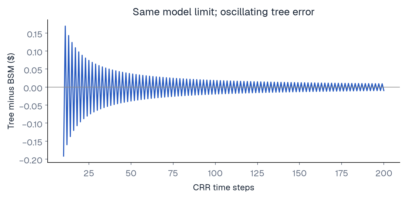
Why oscillation? The payoff has a kink at the strike. Changing the number of steps changes where terminal stock nodes land relative to that kink. A finer grid does not guarantee that every adjacent approximation moves monotonically closer.

Compare several step counts, including even and odd sequences. Look at the size of the error, not just whether the last two prices agree. For early exercise, also inspect the exercise boundary. A single converged European benchmark does not validate every American or barrier implementation.

Barriers introduce another alignment problem. A tree that only checks the barrier at grid times implements discrete monitoring. A contract monitored continuously can knock out between those times. Increasing $N$ helps, but the contractual monitoring rule must be represented deliberately.

A compact implementation

The lab stores only one time slice of option values. That gives $O(N)$ working memory for the plain vanilla recursion. It still visits roughly $N^2/2$ nodes, so the runtime is $O(N^2)$. Recombination saves much more than it eliminates.

Read the terminal payoff first, then the discounted expectation, then the exercise maximum. Each line should correspond to a cash-flow or decision argument. Add discrete dividends, path state, or multiple assets only after explaining why the current state is insufficient.

A tree is a strong choice for a one-dimensional exercise problem and a useful teaching bridge from replication to continuous time. It becomes cumbersome when a contract needs several interacting state variables or a large amount of path history. That is where other numerical methods earn their place.

Try it

For a two-step tree, calculate all three terminal stock prices and call payoffs by hand. Discount the two middle nodes, then today. Now replace the call with a put and compare exercise with continuation at every node. Identify exactly which node changes value; do not simply add an arbitrary premium for being American.

Continue learning

Sources