Brownian motion explained: properties, simulation and quadratic variation

Published 15 October 20266 min readThe maths behind quant finance:Part 1Part 2Part 3 Part 4 Part 5 Part 6

Brownian motion, also called a Wiener process, is a continuous random process whose increments are independent and normally distributed, with variance equal to elapsed time. It is the source of noise in many diffusion models used for pricing and risk.

The practical point is its time scaling. Over an interval of length

\Delta t

, a Brownian increment has standard deviation

\sqrt{\Delta t}

. That makes squared increments accumulate into a nonzero quantity even as the observation grid becomes finer. This is why Itô’s lemma has an extra term.

We will build a finite-grid simulation, examine what it does and does not represent, and calculate quadratic variation. All figures use synthetic Gaussian draws. No historical prices are fitted.

The definition of standard Brownian motion

A standard Brownian motion $W_t$ starts at $W_0=0$ , has continuous paths, and satisfies two increment properties:

For $s<t$ , $W_t-W_s\sim N(0,t-s)$ .
Increments over disjoint time intervals are independent.

The variance convention fixes its scale. In particular, $W_t\sim N(0,t)$ , so its standard deviation at time $t$ is $\sqrt t$ . A process $\sigma W_t$ has variance $\sigma^2t$ .

“Continuous paths” means the model has no jumps. It does not mean paths are smooth. Brownian paths are almost surely nowhere differentiable. Drawing straight lines between simulated observations is a display choice; it does not turn those connecting lines into the true continuous path.

Do not confuse independent increments with independent values. $W_1$ and $W_2$ share the increment from 0 to 1, so they are dependent. In fact, for $s\leq t$ ,

\operatorname{Cov}(W_s,W_t) =\operatorname{Cov}(W_s,W_s+W_t-W_s)=s.

More generally, the covariance is $\min(s,t)$ . Independent values at each date would produce a different process with a different path structure.

Why square-root time matters

Take time in years. A one-year Brownian increment has standard deviation 1. A quarter-year increment has standard deviation $\sqrt{0.25}=0.5$ . If a return model uses annualised volatility $\sigma=20\%$ per square-root year, the quarter-year random return component has standard deviation $0.2\times0.5=10\%$ .

For a trading-day convention of 252 days per year, its one-day scale is $0.2/\sqrt{252}\approx1.26\%$ . The calendar convention and the model both matter. Actual market returns need not have independent increments or constant volatility, so the scaling is a consequence of this model rather than an empirical law for every asset and horizon.

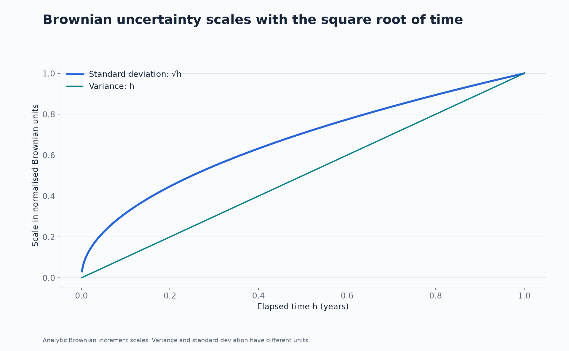
Brownian standard deviation grows as the square root of elapsed time while variance grows linearly; the two scales have different units

The distinction between drift and noise is already visible. A deterministic drift contributes $\mu\Delta t$ . Brownian noise contributes a random term with typical size $\sigma\sqrt{\Delta t}$ . At very short horizons, the latter decays more slowly. This does not mean the noise is always larger on every realised interval; it compares scales across repeated draws.

Units help: if time is in years, $dW$ has square-root-year units, $\mu$ has inverse-year units, and an annualised volatility coefficient has inverse-square-root-year units when multiplying a proportional return.

How to simulate Brownian motion in Python

On an equally spaced grid, independently draw $Z_i\sim N(0,1)$ and set

\Delta W_i=\sqrt{\Delta t}\,Z_i,\qquad W_{t_k}=\sum_{i=1}^{k}\Delta W_i.

For an irregular grid, replace $\Delta t$ with each actual interval length. The starting value belongs in the output, and the cumulative sum must run along the time axis.

The following experiment checks the endpoint variance across independent paths. The output is a random-sample check, not an equality imposed by the code:

import numpy as np

rng = np.random.default_rng(20261015)
paths, steps, horizon = 20_000, 100, 1.0
increments = rng.normal(0.0, np.sqrt(horizon / steps), (paths, steps))
terminal = increments.sum(axis=1)
print(f"mean={terminal.mean():.4f}, variance={terminal.var(ddof=1):.4f}")
# mean=0.0021, variance=1.0044

The downloadable package records the executed output and includes the figures at a finer grid. Use separate path and time axes when extending the example: averaging endpoints estimates a distributional moment; averaging one path through time answers a different question.

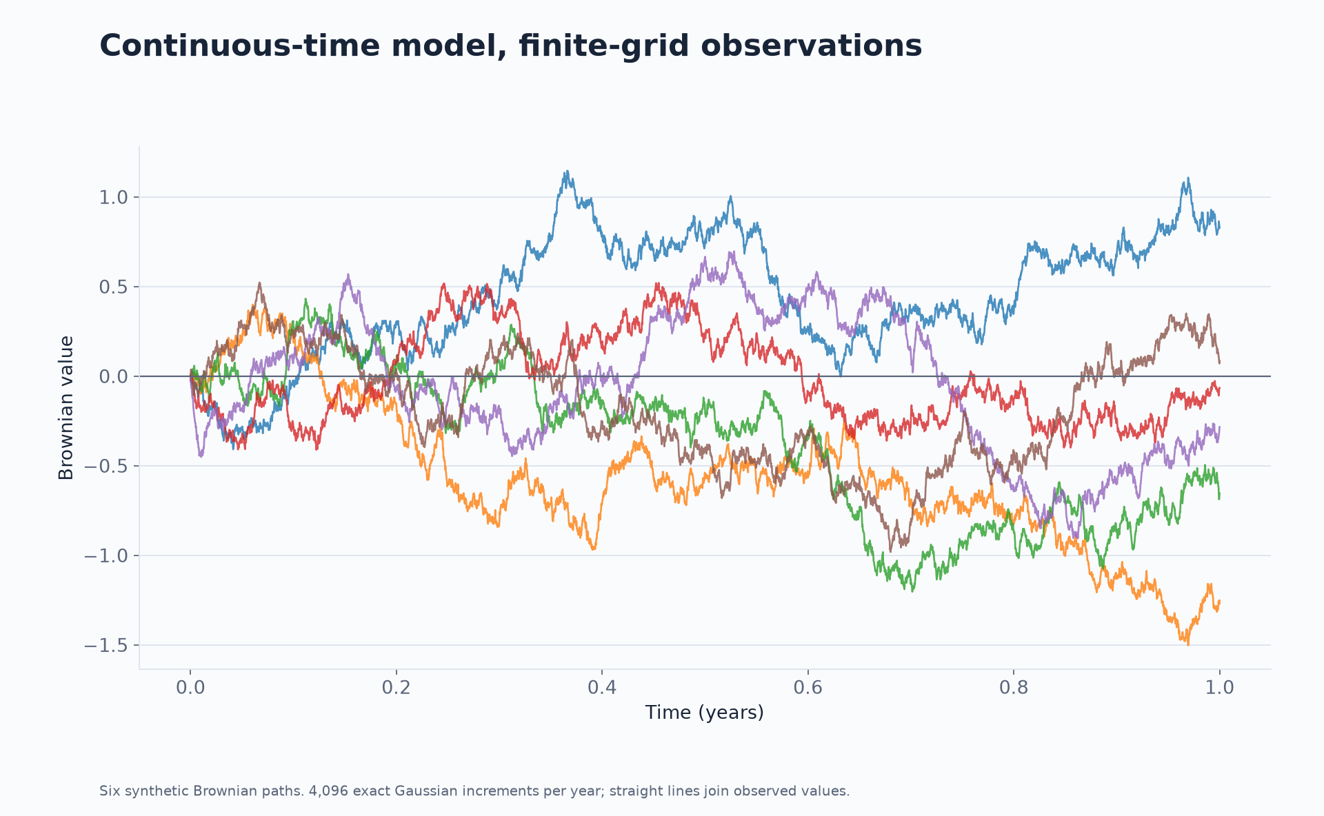
Six synthetic Brownian motion paths observed on a grid of 4096 intervals over one year; connecting segments are display aids

These increments generate the exact joint Brownian distribution at the chosen dates. There is no Euler approximation error in those grid values. But the simulation does not explicitly generate every point between dates. If a payoff depends on a barrier crossing between observations, checking only the grid can miss it.

Drawing more paths reduces sampling uncertainty about a grid-based calculation. Adding more observation dates changes what you can resolve within each path. These are separate operations.

Brownian motion as a scaled random walk limit

Consider a symmetric random walk with $n$ independent steps over one unit of time. Give each step size $1/\sqrt n$ rather than 1. Its endpoint variance is then

n\left(\frac1{\sqrt n}\right)^2=1.

Without the scaling, endpoint variance would grow with $n$ . With it, the distribution has a meaningful limit. A functional limit theorem, under its usual assumptions, turns the appropriately interpolated random walks into Brownian motion in distribution as processes. An endpoint central limit theorem by itself establishes only an endpoint statement.

This is useful intuition for the noise scale, but a Gaussian-increment simulation is simpler when Brownian motion itself is the target. A finite binomial walk is still discrete; it is not literally a Brownian path.

Quadratic variation: why squared noise survives

For a partition $0=t_0<\cdots<t_n=T$ , define

Q_n=\sum_{i=0}^{n-1}(W_{t_{i+1}}-W_{t_i})^2.

On an equal grid, each increment has variance $T/n$ . Therefore $\mathbb E[Q_n]=T$ . A centred Gaussian with variance $v$ has squared-value variance $2v^2$ . Independence gives

\operatorname{Var}(Q_n)=n\times2(T/n)^2=\frac{2T^2}{n}.

The mean stays at $T$ while the variance tends to zero. Hence $Q_n\to T$ in mean square, and therefore in probability, on these deterministic grids. For general deterministic partitions, the variance is $2\sum_i(\Delta t_i)^2$ , bounded above by $2T$ times the largest interval; the same conclusion follows as the mesh tends to zero.

This is a convergence statement about a sum. It does not say that each realised squared increment equals its interval length. A particular Gaussian increment may be tiny or large. Replacing every finite $\Delta W_i^2$ with $\Delta t_i$ would erase genuine variation.

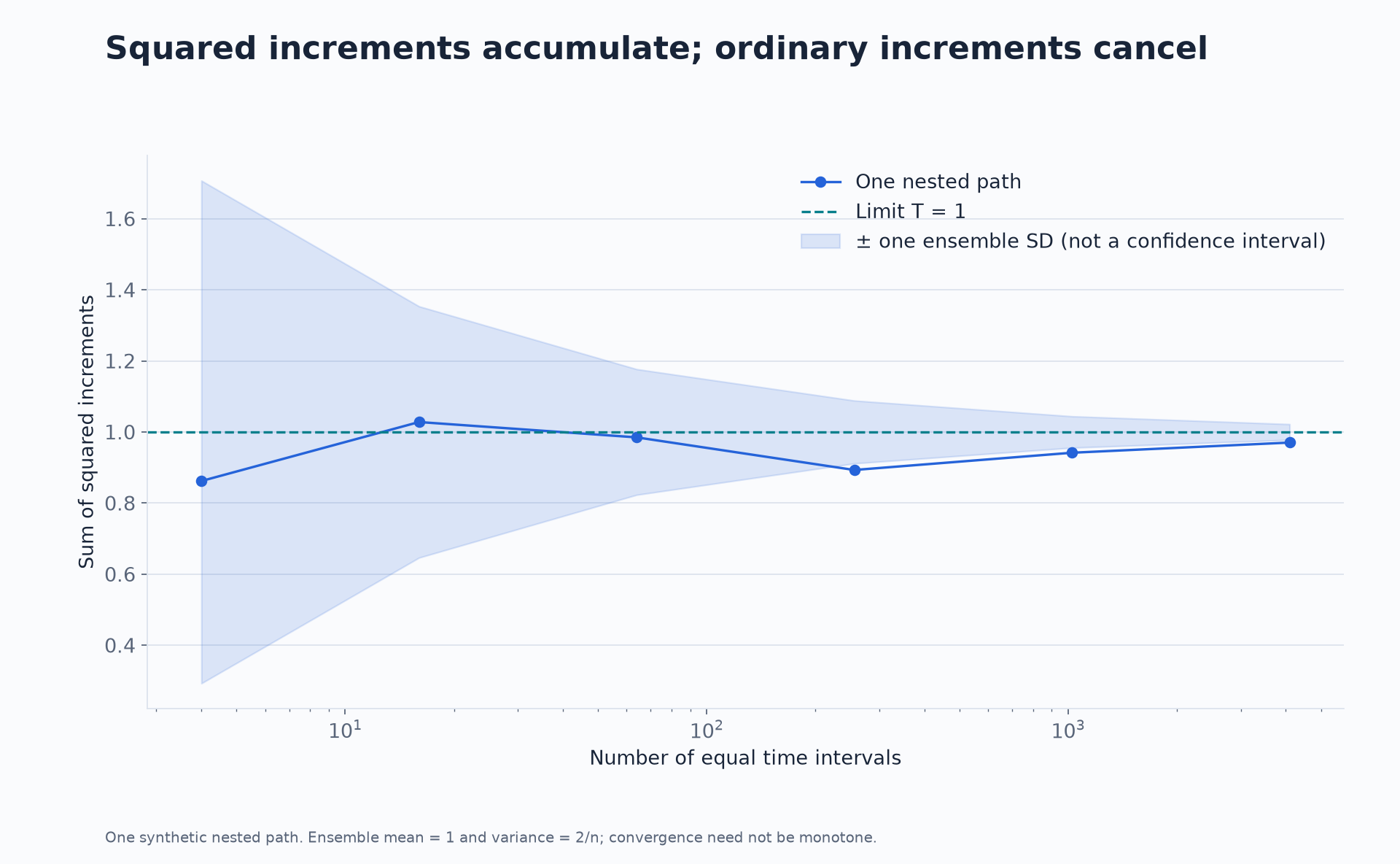
One nested Brownian path’s squared-increment sums approach the one-year quadratic variation target; convergence can fluctuate rather than improve monotonically

The shaded band in the chart is the ensemble mean plus or minus one ensemble standard deviation, $1\pm\sqrt{2/n}$ . It is not a confidence interval for an estimated parameter, and it is not a guarantee that this one path stays inside the band.

To compare time grids fairly, the figure aggregates increments from one common fine path. Generating a fresh unrelated path at every grid size would mix path-to-path variation with the effect of partition refinement.

Where ordinary calculus breaks

For a smooth function, a second-order Taylor expansion contains $\tfrac12 f''(W)(\Delta W)^2$ . In ordinary calculus with a smooth input, squared increments vanish when accumulated over an increasingly fine partition. For Brownian input, their sum tends to elapsed time.

That surviving second-order term produces the Itô correction. The notation $(dW)^2=dt$ is a useful mnemonic for this result. It is not an algebraic identity between infinitesimal random variables.

For example, ordinary chain-rule reasoning would suggest $d(W_t^2)=2W_t\,dW_t$ . The correct Itô expression is

d(W_t^2)=2W_t\,dW_t+dt.

Taking expectations gives $\mathbb E[W_t^2]=t$ , which matches the known Gaussian variance. Omitting $dt$ would incorrectly predict a zero expected square.

The next article derives this carefully and applies it to log stock prices and exponential functions.

What Brownian motion does not model by itself

Brownian motion can be negative, so directly setting a stock price equal to

100+\sigma W_t

permits negative prices. Geometric Brownian motion exponentiates a related process to preserve positivity, while introducing its own assumptions.

Gaussian independent increments also exclude jumps, volatility clustering and many forms of serial dependence. Brownian motion remains useful as a building block inside richer models, but choosing the driver does not establish that the whole model fits a particular asset.

For several assets, independent Brownian drivers imply zero instantaneous correlation. Correlated drivers require a valid positive-semidefinite covariance structure; copying the same noise into every asset instead gives perfect correlation. A factorisation or explicit factor construction can impose the intended dependence.

Finally, Brownian motion is a martingale with respect to its natural information flow. That fact concerns conditional means. It does not make a nonlinear function of Brownian motion a martingale automatically, as the square example demonstrates.

A useful checkpoint

Suppose $T=2$ and you use 200 equal intervals. Each increment must have variance $0.01$ and standard deviation $0.1$ . Using standard deviation $0.01$ would make the endpoint variance $200\times0.01^2=0.02$ , one hundred times too small.

The endpoint target is mean zero and variance 2. The quadratic-variation target is also 2, but it is a different random calculation: a sum of squared increments on one path rather than the squared endpoint averaged across paths.

Being able to distinguish those quantities is a stronger simulation check than producing a plausible-looking squiggle.

Continue learning and download the experiments

The series download includes the path generator, nested quadratic-variation experiment, chart sources and numerical outputs. Run it before changing the time horizon or volatility so you have a known baseline.

For a guided course, start the Options Pricing programme, particularly stochastic processes, Brownian motion and Itô’s lemma. If the probability assumptions are unfamiliar, first use the beginner quant roadmap.

Sources and further study

MIT’s Advanced Stochastic Processes notes cover Brownian motion and quadratic variation. NumPy’s Generator documentation explains the random-generation interface used here. The calculations and simulations above are original teaching examples.