Implied volatility vs historical volatility: what each one measures
Compute historical volatility from returns and implied volatility from an option price, then see why the two differ and how traders compare them.
Implied volatility vs historical volatility: what each one measures
Published 5 min read
Historical volatility measures how much an asset's price has moved: it is the annualised standard deviation of past returns. Implied volatility is the number that makes an option-pricing model match an option's market price, so it describes what the market charges for future movement. One looks backwards at data; the other is read off a price today. The gap between them is information, not an error.
Traders compare the two constantly. An option looks "expensive" when its implied volatility sits well above recent realised volatility, and "cheap" when it sits below. That comparison is useful only if you know how each number is built and what each one leaves out. This guide computes both from scratch.
How do you calculate historical volatility?
Historical volatility, also called realised volatility, starts from daily returns. Take ten daily returns:
Their sample standard deviation is 0.955% per day. To annualise, multiply by the square root of the number of trading days in a year:
σannual=σdaily×252=0.955%×15.87≈15.2%.
The square root comes from adding independent daily variances. A year's variance is 252 times a day's, so its standard deviation is √252 times larger.
Three choices change the answer, and published figures rarely state all of them:
The window. Ten days, 30 days and one year give different numbers for the same asset.
The mean. Many practitioners subtract nothing and use the root mean square of returns, because the average daily return is tiny and noisy. On these ten returns that gives 14.4% instead of 15.2%.
The data. Close-to-close returns ignore what happened during the day. Estimators that use the open, high, low and close can be more efficient, but they are sensitive to microstructure noise.
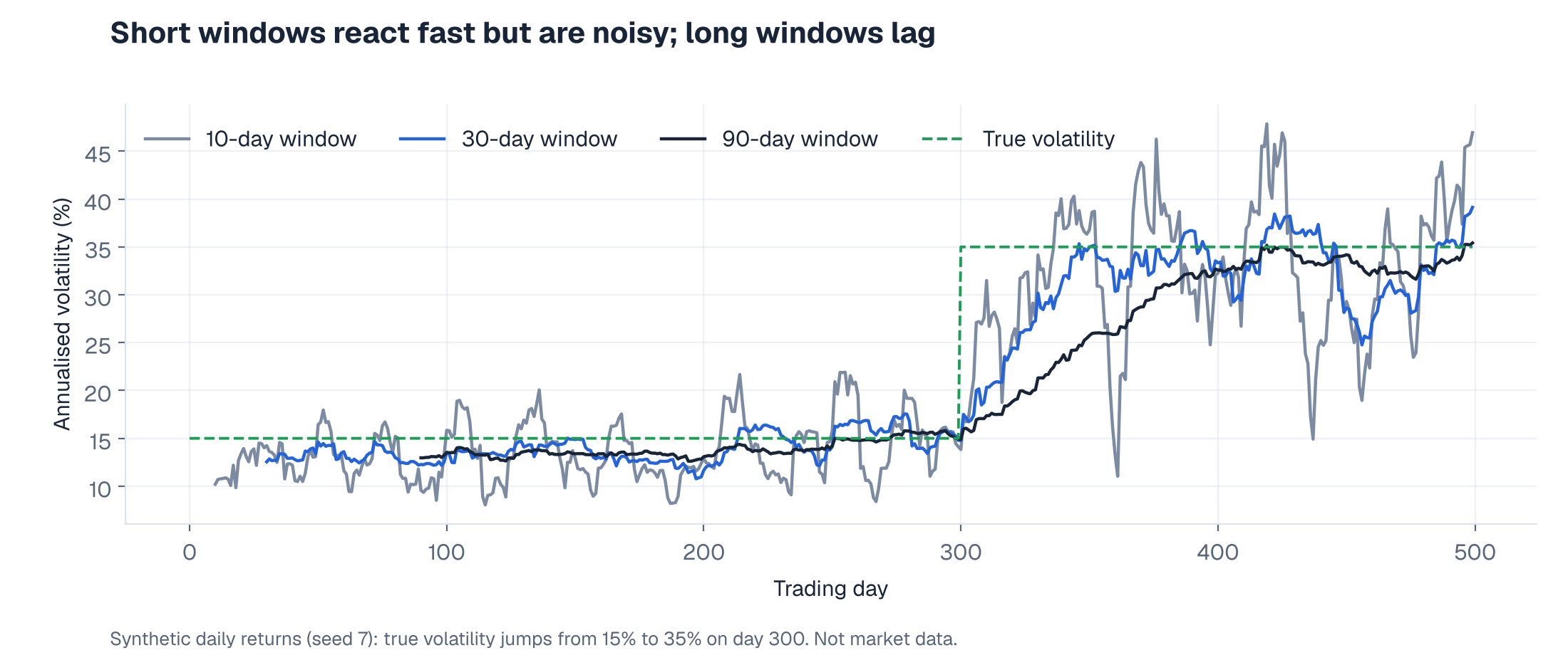
Rolling 10-, 30- and 90-day realised volatility on a synthetic path whose true volatility jumps from 15% to 35%
The chart shows the window trade-off on synthetic data with a known answer. When true volatility jumps from 15% to 35%, the 10-day estimate reacts within days but swings widely. The 90-day estimate is smooth, but it takes months to catch up. No window is right; each answers a different question about the past.
How do you get implied volatility from an option price?
Implied volatility runs the pricing model backwards. Black–Scholes takes spot, strike, time, rates and volatility and returns a price. Every input except volatility is observable, so we search for the volatility that reproduces the market price.
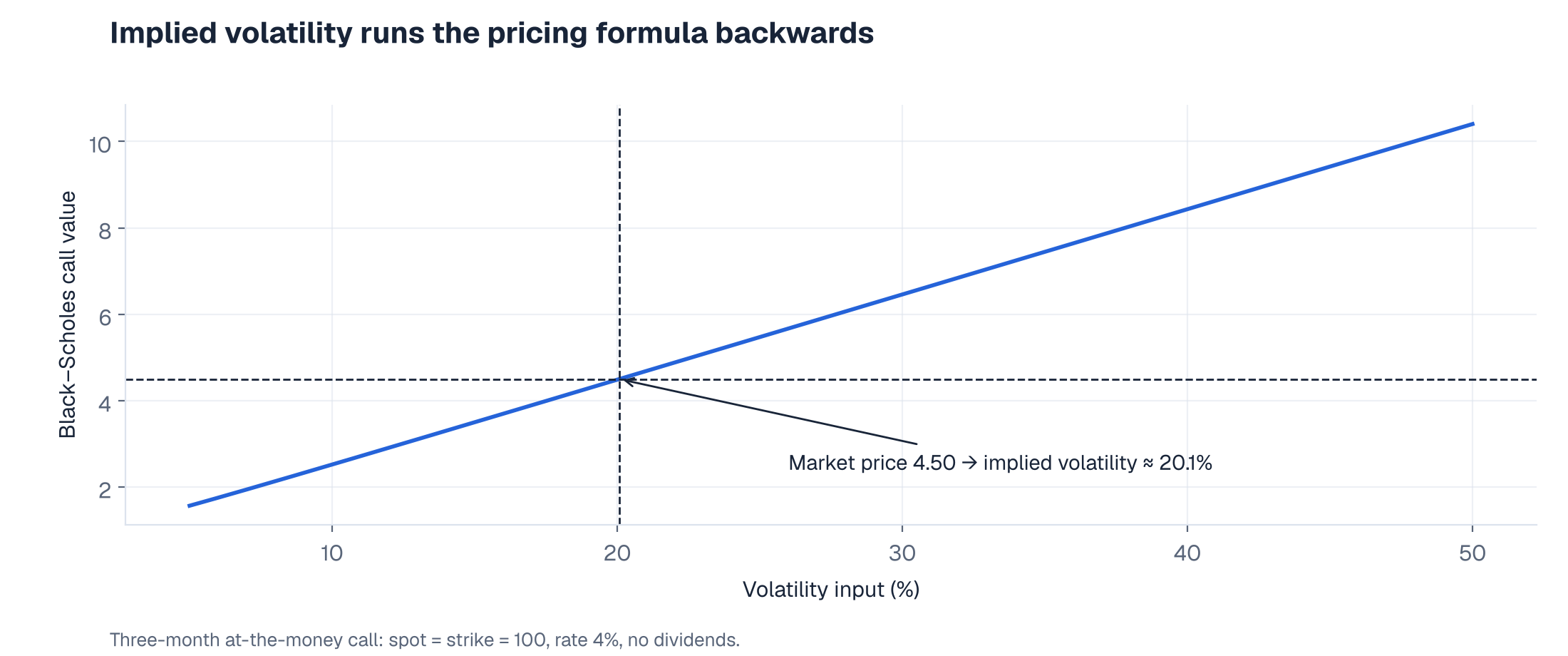
Suppose a three-month at-the-money call on a 100stocktradesat4.50 with a 4% rate. Black–Scholes gives 4.49at203.50, the implied volatility would be 15.0%.
Black–Scholes call value against the volatility input, with a market price of 4.50 mapping to 20.1%
Because price rises with volatility, the answer is unique, and quoting options in implied-volatility terms lets traders compare contracts with different strikes and expiries on one scale. That is why option desks quote "vol" rather than dollars.
You can do the forward direction yourself in the Black–Scholes option pricing calculator: fix the other inputs, then move volatility until the price matches a quote.
What does a volatility number mean in price terms?
An annualised volatility converts to a typical move with the same square-root rule. At 20%:
a one-day standard deviation is 20% / √252 ≈ 1.26%;
a 30-calendar-day standard deviation is 20% × √(30/365) ≈ 5.73%.
So a stock with 20% implied volatility is priced as if a one-standard-deviation move over the next month is about ±5.7%. This is a rough guide, because real returns have fatter tails than the normal distribution behind the rule.
Why do implied and historical volatility differ?
They measure different things, so they should differ.
Different time periods. Historical volatility describes the past window. Implied volatility describes the option's remaining life, so it should anticipate known events such as earnings, central-bank meetings and elections. Implied volatility on a stock often rises into an earnings date and falls straight after it.
A risk premium. Sellers of options take on crash risk and must be paid for it. For equity index options, implied volatility has on average exceeded the volatility later realised, a gap called the variance risk premium (Carr and Wu, 2009). It is an average, not a rule: in a sudden crash, realised volatility can far exceed what was implied beforehand.
The smile. One asset has many implied volatilities: one per strike and expiry. Low-strike equity index puts usually trade at higher implied volatility than at-the-money options. A single historical number cannot match all of them. The volatility surface explorer shows how skew and term structure shape that set.
Model assumptions. Implied volatility is defined through Black–Scholes. If the market prices jumps, stochastic volatility or supply and demand for particular strikes, all of that is absorbed into the one number the model allows to vary.
How do traders use the comparison?
The common comparison is implied volatility today against a forecast of realised volatility over the option's life, not against the last month's realised figure. The question is whether the option's price pays enough for the movement you expect.
A delta-hedged long option earns, roughly, the difference between the variance that is realised and the variance that was implied, weighted by its gamma along the way. Buy an option at 20% implied, hedge it, and see 25% realised: you tend to profit. See 15% realised and the time decay wins. This is the logic behind volatility trading and why forecasting realised volatility well is valuable.
Three cautions apply:
A forecast from a 30-day window is just one estimate. GARCH-type and EWMA models weight recent days more heavily and usually forecast better than a flat window.
Hedging is discrete and costs money, so the theoretical edge shrinks in practice.
The variance risk premium is compensation for real risk. Selling volatility looks profitable in calm years and can lose years of gains in one crash.
Common mistakes
Mixing calendar and trading days. Annualise daily returns with 252 trading days. Express option time in calendar days over 365, as the pricing calculator does. Annualising daily returns with √365 instead of √252 overstates volatility by about 20%, because √(365/252) ≈ 1.20.
Comparing at the wrong maturity. A 30-day historical figure should be compared with 30-day implied volatility, not with a one-year option.
Treating implied volatility as a forecast. It is a price. It contains a forecast, a risk premium and the effects of supply and demand, and these cannot be separated without a model.