GARCH volatility forecasting: persistence, mean reversion and a forecast you can audit

Published 14 October 20264 min readVolatility forecasting and risk:Part 1 Part 2 Part 3Part 4Part 5 Part 6 Part 7 Part 8 Part 9 Part 10

After a large market move, tomorrow's uncertainty may rise. It need not stay at that level indefinitely. A GARCH model connects those two ideas: recent shocks affect the next variance forecast, while the variance process can revert towards a longer-run level under stated parameter conditions.

That extra structure can be useful. It also gives us parameters to estimate, assumptions to inspect and another opportunity to confuse a fitted curve with a genuine forecast.

Write down the recursion

In a zero-mean GARCH(1,1) example, let Rₜ = √hₜ Zₜ, with standardised shocks having mean zero and variance one. The variance update is:

h_{t+1}=\omega+\alpha R_t^2+\beta h_t.

For this conventional specification, positive ω and nonnegative α and β preserve positive conditional variance. The additional condition α + β < 1 gives a finite unconditional variance under the usual stationary setup with variance-one innovations.

That finite-variance condition is not the complete theory of strict stationarity, nor does it guarantee a finite fourth moment. Different moment questions have different conditions.

Use ω = 0.000002, α = 0.08 and β = 0.90. Begin with hₜ = 0.0001 and observe a return of −3%:

h_{t+1}=0.000002+0.08(0.0009)+0.90(0.0001)=0.000164.

The next daily volatility forecast is approximately 1.2806%. The long-run variance implied by these parameters is ω/(1 − α − β), or 0.0001.

Persistence governs the forecast path

The sum α + β is 0.98. For horizons beyond the first forecast, the expected squared shock equals the corresponding forecast variance under the model. This produces:

\mathbb E_t[h_{t+k}]=\bar h+(\alpha+\beta)^{k-1}(h_{t+1}-\bar h), \qquad k\ge1.

Here h̄ is the long-run variance. The forecast path approaches that level gradually. A persistence estimate near one implies slow mean reversion and makes the inferred long-run level sensitive to the denominator 1 − α − β.

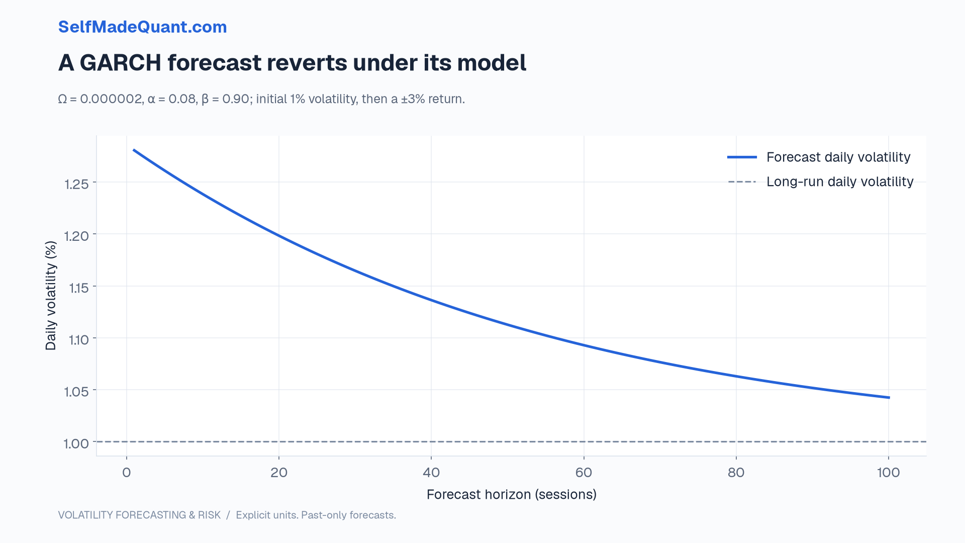
GARCH forecasts after a three per cent shock gradually approach the stated long-run variance

If the model's variance process changes structurally, a previously estimated long-run level can become a poor reference. A parameter constraint does not protect the forecast from a new market regime.

A ten-day forecast requires ten variances

Under the zero conditional mean and uncorrelated-innovation assumptions used here, the variance of the sum of the next ten returns equals the sum of their conditional variance forecasts.

For the example above, that sum is approximately 0.00158537. Its square root is 3.9817%. Simply multiplying the first daily volatility forecast by √10 gives 4.0497%.

The difference comes from forecast mean reversion. It is modest in this invented example, but it demonstrates why horizon aggregation is a model calculation rather than a formatting change.

This sum describes an additive return quantity. Applying it directly to a compounded simple-return portfolio requires another approximation or a path simulation. If the conditional mean has dynamics, its forecast uncertainty can also affect the return variance.

Estimation needs an information boundary

The usual fitting procedure chooses parameters to explain a sample of returns. Under a Gaussian quasi-likelihood, one relevant contribution is log(hₜ) + Rₜ²/hₜ, apart from constants and scaling.

Calling it a quasi-likelihood matters. Using a Gaussian fitting criterion does not establish that the actual return distribution is Gaussian. Consistency arguments require conditions on the mean, variance process and regularity; they do not follow from a successful optimiser status alone.

Our project deliberately uses a coarse, declared grid of sixty candidate parameter combinations. Each candidate has nonnegative coefficients and persistence below one. The fitted initial variance comes only from the current fit sample.

This is an auditable teaching estimator, not a claim to have found the continuous maximum-likelihood solution. A candidate at a grid edge is a diagnostic: a wider or finer search might materially change the result. Production fitting also needs convergence diagnostics, parameter uncertainty and sensitivity to starting values.

Keep percentages and decimals consistent

Suppose you multiply returns by 100 before fitting a library model. Variance is then measured in squared percentage points rather than squared decimal returns.

To convert a variance forecast back to decimal-return variance, divide by 10,000. Divide its standard deviation by 100. The intercept ω changes scale too, while the dimensionless α and β coefficients do not change under this pure rescaling.

This unit check is easy to overlook because both model outputs may look like small positive numbers. In a risk report, the resulting error can multiply a dollar loss threshold by one hundred.

Check the output's date convention

A forecast table can be aligned to its origin or its target. A row labelled Monday might mean a forecast made on Monday for Tuesday, rather than a forecast for Monday made earlier.

The arch documentation explains its origin and target alignment options and its variance forecast outputs. Inspect the convention instead of guessing from a DataFrame index. Forecast output documentation.

The useful final record contains both dates, the forecast horizon, the fit-sample endpoint, parameters and units. Those fields let another person reconstruct what was known before the observation arrived.

Next, we will change the effect of a shock's sign and examine why a correct variance forecast can still understate tail losses.

Continue to asymmetric shocks and heavy tails, or study the full GARCH lesson.

Background: McNeil, Frey and Embrechts, Quantitative Risk Management, Chapter 4. Numerical examples are independently implemented in the accompanying lab.

Subscribe for the series and practise quant interviews.

Until then, peace.