Realised volatility: a flat close can hide a busy day

An asset opens at 100 and closes at 100. Was it a quiet day?

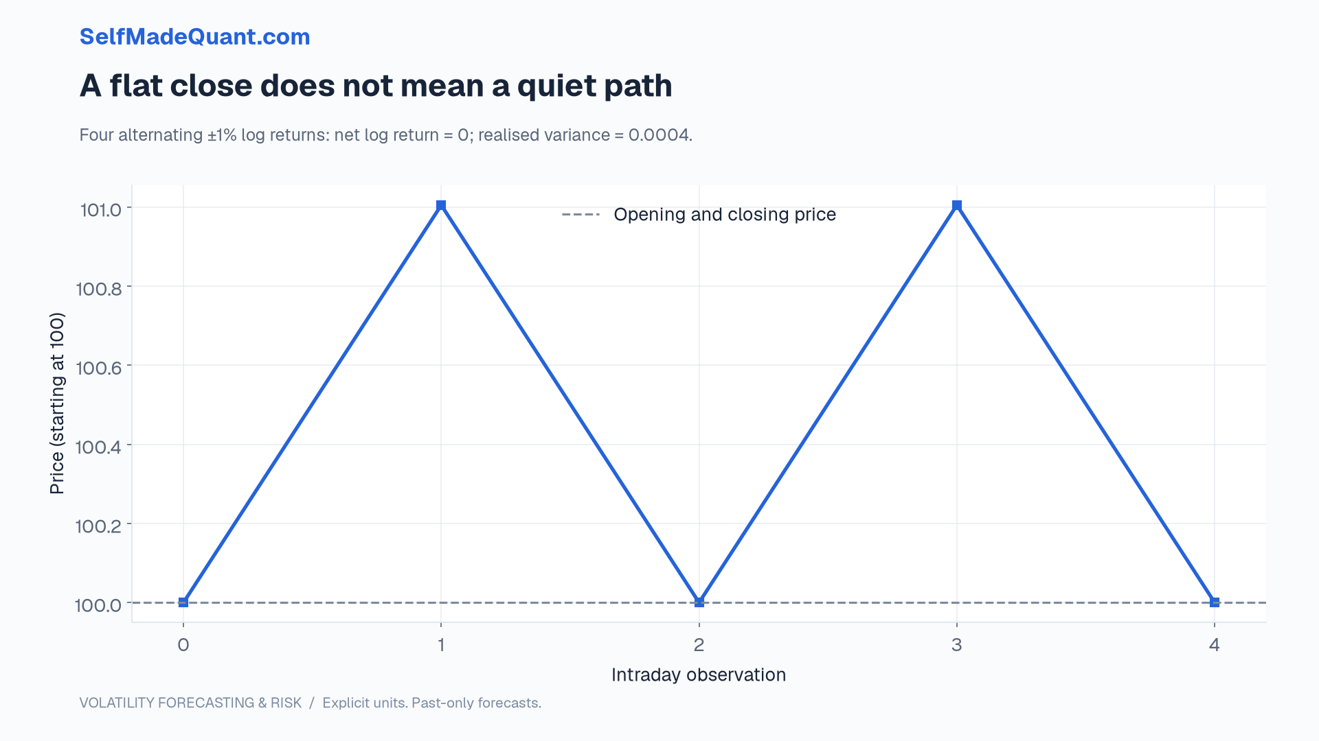
The two endpoints cannot tell you. The asset may have stayed near 100 throughout the session. It may also have moved sharply in both directions before returning to the starting value. A close-to-close return records the net change, not the path taken to reach it.

This distinction matters when you use a completed day's movement to judge a volatility forecast. It also matters when your exposure changes within the day: a strategy can experience substantial intraday losses even though the final price returns to where it began.

Build a deliberately simple path

The sum of squared log returns is different:

Its square root is 2%. This is a measure of variation accumulated along the sampled path. It is not a 2% profit or a 2% loss, and it is not the standard deviation of these four observations with a sample-mean correction.

What the measurement is trying to approximate

For a continuous price process with sufficiently regular volatility and clean observations, increasingly fine squared log-return sums can approximate integrated variance over a fixed interval.

That statement has conditions. If the process jumps, the limiting quadratic variation also includes squared jumps. If observations contain market microstructure noise, the simplest sum can become badly contaminated as sampling becomes finer.

The target therefore belongs beside the measurement. Are you trying to measure continuous variation, total quadratic variation including jumps, or a practical proxy for next-day return variance? Those questions can require different estimators.

Our offline forecasting project uses squared daily returns as its evaluation proxy. It does not pretend to contain intraday quotes or to reconstruct integrated variance from a closing-price file.

More ticks can mean more noise

Suppose an observed log price equals an efficient log price plus independent, mean-zero observation noise with variance η². An observed return contains the change between two noise observations.

That difference has variance 2η². Summing n such squared noise differences produces an expected noise contribution of 2nη². Independence between adjacent differences is not required for this expectation calculation; the shared endpoints matter for other properties.

Set η to one basis point in log-price units, or 0.0001. The noise contribution alone has expectation 0.000002 with 100 intervals, but 0.0002 with 10,000 intervals. Its square root in the second case is about 1.41%.

This is an invented measurement model, not an empirical estimate of a particular exchange. It explains the direction of a problem: sampling more frequently need not improve a naive realised-variance estimate when each observation adds noise.

A practical measurement checklist

Start by stating the session boundaries. A regular-session realised variance and a close-to-close forecast have different coverage. Overnight squared returns can be recorded separately, then combined under a clearly specified convention.

Next, examine what each observation represents. A transaction price can bounce between bid and ask. A midpoint reduces one source of bounce but introduces quote-quality and staleness questions. Neither label guarantees clean data.

Check timestamps, duplicate messages, out-of-sequence records and long gaps. A zero return during a stale-quote interval is not proof that economic uncertainty disappeared. An extreme return around a split may be a corporate-action error. An extreme return around genuine news may be exactly the event the risk model should retain.

Then compare sampling frequencies. A plot of average measured variance against sampling interval can reveal sensitivity. It does not, by itself, identify the true variance or prove which estimator is optimal.

Finally, preserve the raw-to-clean transformations. If an outlier rule removes the largest moves, the evaluated forecast may look well calibrated because the difficult observations were deleted. Data cleaning needs an economic explanation and a reproducible log.

A better proxy still leaves uncertainty

Imagine that a forecast has variance 0.0001. A single squared daily return may be almost zero or many times that value. The observation is noisy even if the forecast is correct on average under the assumed model.

Using richer intraday measurements can reduce some of that noise. It can also add different biases. Comparing forecasts therefore requires matching the proxy to the horizon and understanding how the chosen score responds to measurement error.

The wrong conclusion is that volatility cannot be evaluated because it is latent. The useful conclusion is that the evaluation design needs to describe the proxy, its limitations and the assumptions under which model rankings remain informative.

Before fitting anything, build three columns: observation period, proxy value and availability time. The forecast must precede the period being measured; the proxy can only be used after it becomes available.

Next we will build a forecast that you can calculate by hand, update after each observation and audit without an optimiser.

Until then, peace.