Volatility forecasting: what are you actually predicting?

A risk report says that an asset has 20% volatility. Before using that number to size a position, ask three questions. Twenty per cent of what? Over which horizon? Estimated with information available when?

Those questions change the amount of capital you might commit. They also separate a description of yesterday's movement from a forecast of tomorrow's uncertainty.

This series builds a complete volatility research workflow. We will measure returns, compare forecasts, turn a distribution into loss thresholds, and test how the resulting risk decisions behave when assumptions fail. The final Python project runs offline, so every reported number can be reproduced.

Start with a return and a clock

Let an adjusted asset value move from 100 to 101 over one trading session. Its simple return is 1%. Its log return is log(101/100), approximately 0.995%.

Simple returns connect directly to a fixed position's profit. Log returns add over time. They agree approximately for small movements, but they are not interchangeable labels for the same observation.

If an asset rises 10% and then falls 10%, its value moves from 100 to 110 to 99. Adding the simple returns gives zero; compounding gives a 1% loss. Adding the log returns correctly produces log(0.99).

Write your convention into the dataset. An adjusted total-return series, an unadjusted price series and a futures settlement series can encode different economic quantities. A dividend or stock split can create a misleading return if the adjustment convention is wrong. A futures roll can introduce a move that belongs to the contract construction rather than the market exposure you intended to measure.

The clock matters too. A close-to-close return includes overnight movement. An open-to-close return does not. If your position spans the night, a model trained only on intraday returns leaves out part of the exposure.

Variance describes dispersion around a mean

For a return R, variance is the expected squared deviation from its mean. Volatility is its square root:

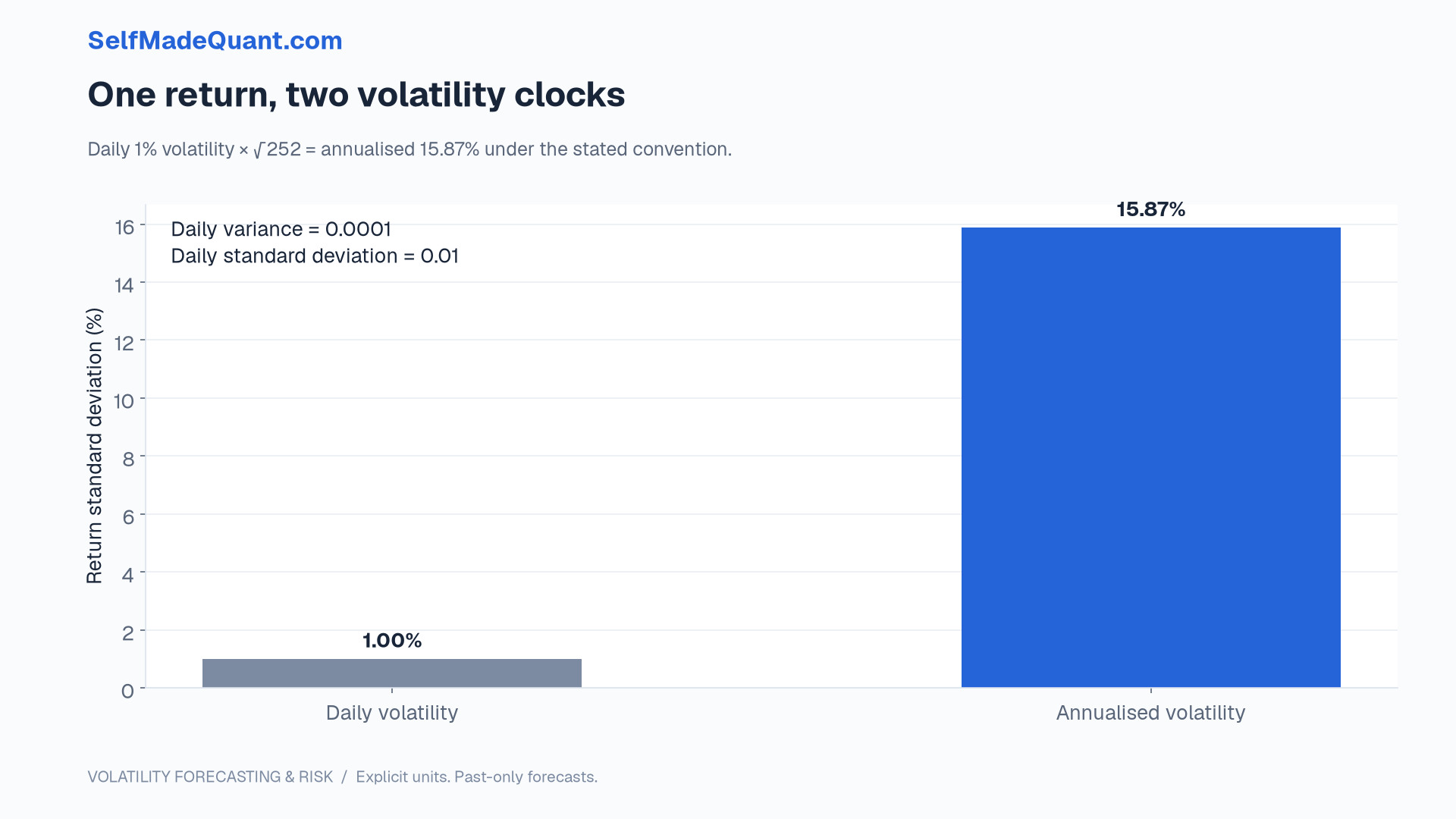
The units are different. Decimal-return variance might be 0.0001. Its volatility is 0.01, or 1%. Reporting 0.0001 as though it were a 0.01% volatility estimate introduces a unit error before the forecasting problem has even started.

Suppose the daily standard deviation is 1%. Multiplying it by the square root of 252 gives approximately 15.87% annualised volatility. The number 252 is a stated trading-session convention. It is not a claim that the next calendar year will contain exactly that many relevant observations for every instrument.

The square-root rule follows from adding variances when the returns being added have no serial covariance and comparable variance. With changing conditional variances, forecast the relevant sequence of variances. With serial correlation, include covariance terms. Neither situation is repaired by automatically multiplying one daily estimate by a square root.

Historical, realised and forecast volatility answer different questions

Historical volatility usually summarises past returns over a chosen window. It is an estimate, affected by the window, the mean convention and the observations included.

Realised variance commonly sums squared intraday log returns over a completed period. Under appropriate assumptions it is a useful proxy for variation during that period. It is still measured with data and sampling choices, rather than observed directly without error.

A conditional variance forecast asks a different question: how much variation do we expect next, given the current information set?

Write that forecast as:

The second subscript records the information date. A forecast for Tuesday made after Monday's close may use Monday's return. It may not use Tuesday's completed return, even if the dataset already contains it when you run the notebook months later.

The realised Tuesday return will not equal the forecast standard deviation. A 1% volatility forecast can coexist with a 0.1% return or a 4% return. Judging the forecast requires repeated, correctly aligned observations and a loss function that matches the target.

Implied volatility carries a pricing context

An option's implied volatility is the volatility input that makes a stated pricing model match its market price, given the other inputs. It depends on the option, expiry and pricing convention. Different strikes can imply different values.

Do not treat an implied-versus-realised difference as automatic profit. You must specify the instrument, the payoff, the pricing measure, execution costs and the risks carried between observations. An option premium can compensate a seller for exposures that a simple variance comparison leaves out.

A volatility estimate is one input to risk

Two positions can have the same return volatility and very different losses under a large price move. A short option, an illiquid leveraged holding and an unleveraged liquid stock have different payoff and funding structures.

Even for a linear position, standard deviation does not describe which side of the distribution contains the extreme outcomes. It does not determine how quickly you can sell, whether funding remains available or what happens when a hedge stops behaving as expected.

The practical first task is to write a forecast contract: instrument, return definition, horizon, units, information timestamp, forecast target and intended decision. If those fields are missing, a more sophisticated model can make the ambiguity harder to spot.

Next, we will examine what a completed day actually tells us about volatility, and why increasing the number of observations can sometimes make the measurement worse.

Until then, peace.