EWMA volatility forecasting: how quickly should yesterday change your risk estimate?

Published 14 October 20264 min readVolatility forecasting and risk:Part 1 Part 2Part 3Part 4 Part 5 Part 6 Part 7 Part 8 Part 9 Part 10

Your daily volatility estimate is 1%. The next observed return is −3%. How much should your forecast rise?

Keeping the old estimate ignores new information. Replacing it with 3% gives one observation complete control. An exponentially weighted moving average, or EWMA, provides a transparent compromise: retain part of the old variance and add part of the new squared shock.

The useful feature is the update you can inspect. It also makes the model's limitations unusually visible.

Update variance before taking a square root

Let hₜ be the variance forecast made for period t using earlier information. Let εₜ be the observed return minus the mean forecast that was available before that return. For a decay parameter λ between zero and one:

h_{t+1}=\lambda h_t+(1-\lambda)\epsilon_t^2.

We will assume a zero conditional mean in the numerical example. That makes εₜ equal to the return. It is an explicit modelling choice, not an instruction to ignore a meaningful mean in every dataset.

Use λ = 0.94, hₜ = 0.0001 and εₜ = −0.03. The update is:

h_{t+1}=0.94(0.0001)+0.06(0.0009)=0.000148.

The next daily volatility forecast is approximately 1.2166%. Averaging 1% and 3% directly would produce a different result because volatility is the square root of variance. The recursion operates on squared returns.

The sign disappears when the shock is squared. A +3% observation gives exactly the same update as −3%. We will later add a mechanism that allows the signs to have different effects.

What the decay parameter actually does

Repeated substitution shows that past squared shocks receive geometrically declining weights. A shock from j updates ago has a coefficient proportional to λʲ.

With λ = 0.94, the weight of a particular shock halves after approximately:

\frac{\log(0.5)}{\log(0.94)}=11.20

updates. This is the half-life of its weight. It is not a promise that the forecast itself will return halfway to its starting value in eleven sessions. New observations arrive during those sessions and change the forecast too.

A shock receives geometrically declining EWMA weight; its weight half-life differs from the forecast's realised recovery

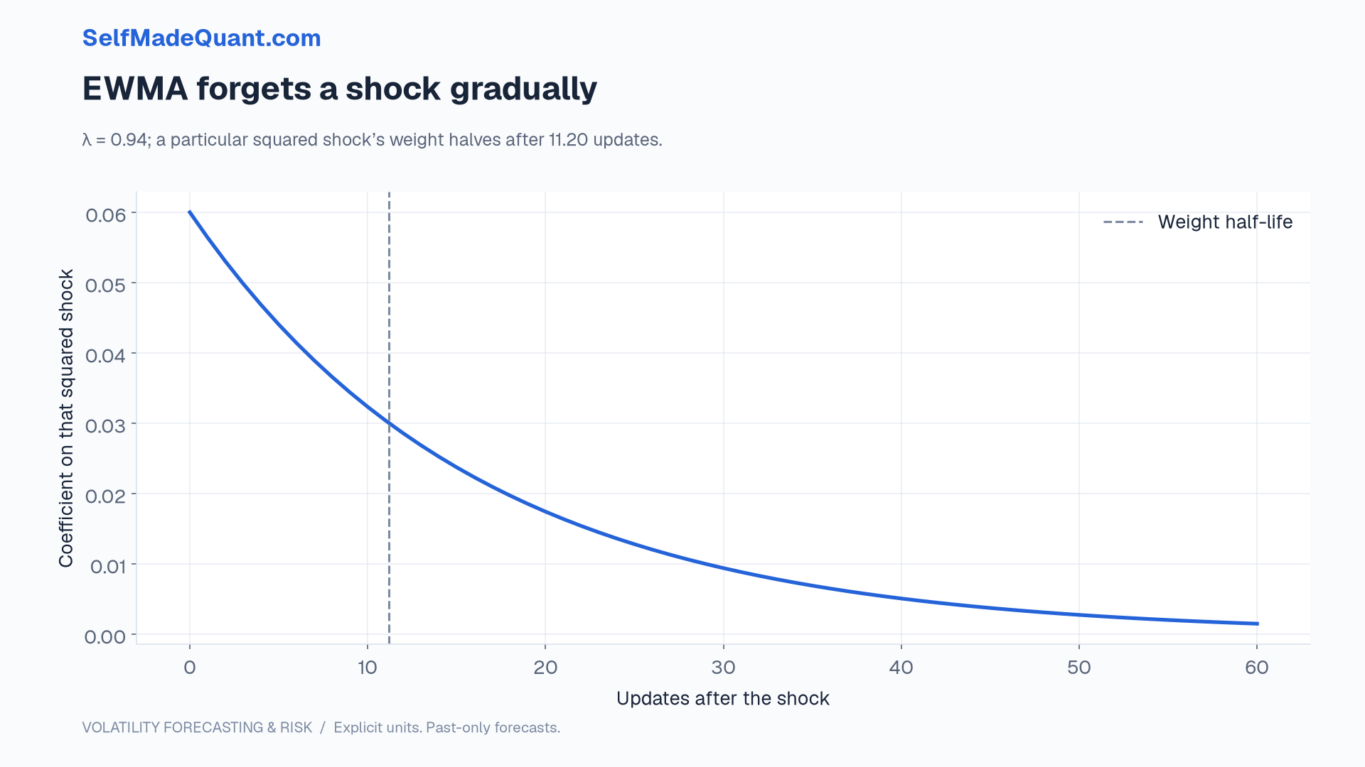
A smaller λ reacts more quickly and forgets more quickly. A larger λ smooths more heavily. Neither is universally better: a fast response can help after a variance change while allowing isolated noisy observations to move the estimate more.

The value 0.94 is a useful teaching example. It should not become an unexplained constant in every strategy. Our final project compares 0.90, 0.94, 0.97 and 0.99 on a development-validation block, then freezes the selected value before the final evaluation.

Contrast a rolling window

A rolling twenty-session mean of squared returns assigns equal weight to the twenty observations inside its window and zero weight to everything outside it.

That can create a sharp drop when a large shock leaves the window, even if today's return is ordinary. EWMA removes that particular cliff by reducing weights gradually.

It does not follow that EWMA must forecast better. The rolling window can be a strong baseline, and its behaviour may fit a particular change pattern. Comparing the methods requires the same dates, units, forecast horizon and information set.

Do not compare a twenty-day rolling standard deviation using a fitted mean with a zero-mean EWMA second moment and silently attribute every difference to weighting. Specify both the weighting rule and the treatment of the mean.

Initialisation leaves a trace

The recursion needs an initial variance. You can estimate it from a training sample, use a prespecified value or apply a documented backcast. Different choices can matter near the beginning of the series.

After k updates, the initial value's coefficient is λᵏ. That gives you a direct way to assess how much initialisation remains in the forecast. A warm-up period can reduce its influence, but the warm-up data must themselves have been available at the relevant forecast origin.

In an out-of-sample experiment, initialising with the full dataset's variance leaks later information. The state may look reasonable, yet the forecast has borrowed a summary statistic from the future.

Our project estimates the initial second moment from the available fit sample and replays that sample before scoring later observations. Those early states are in-sample quantities; we do not label them out-of-sample forecasts.

A forecast clock you can test

For a forecast of session t, append the current variance to the output before incorporating return t:

def ewma_forecasts(returns, initial_variance, decay=0.94):
    variance = initial_variance
    forecasts = []
    for observed_return in returns:
        forecasts.append(variance)
        variance = decay * variance + (1 - decay) * observed_return**2
    return forecasts

print(ewma_forecasts([-0.03], 0.0001))
# [0.0001]

That single ordering decision determines whether the output predicts the observation or already knows it. The next state after the example observation is 0.000148; the forecast for that observation was 0.0001.

What EWMA leaves unspecified

The update has no separate long-run variance anchor. If you use its forecast distribution recursively with zero mean, the expected future variance remains at the current level. Actual future observations will still move the estimate.

EWMA also does not specify a complete return distribution. A variance forecast alone cannot tell you a 99% loss quantile until you add assumptions about the standardised shocks.

These are reasons to state the model's job carefully. It is a simple, auditable variance forecast, useful as a benchmark and potentially as part of a risk process. Next we will add an intercept and a mean-reversion mechanism, then check what those extra parameters require.

Continue to GARCH. Background: McNeil, Frey and Embrechts, Quantitative Risk Management, Chapter 4, especially exponential-smoothing forecasts; Engle's Nobel lecture provides the broader conditional-volatility context.

Subscribe for the series and practise quant interviews.

Until then, peace.