What maths do you need for quant finance? A guide by task and role

Published 15 October 20267 min readStart learning quant:Part 1 Part 2 Part 3 Part 4Part 5Part 6 Part 7

The main mathematical foundations for quant finance are algebra, calculus, linear algebra, probability, statistics, optimisation and numerical methods. Later priorities depend on the work: empirical research emphasises inference and time series; derivatives pricing adds stochastic processes and calculus; portfolio work uses covariance and constrained optimisation. You can start small projects before mastering every advanced topic.

A useful test is whether you can connect a mathematical object to a financial question. What does a covariance matrix describe? What is uncertain in a Monte Carlo estimate? Which sensitivity is a derivative measuring? A familiar formula is less useful if you cannot explain the quantity it produces.

This guide maps subjects to tasks and gives two worked examples. For a complete study sequence, use the quant roadmap.

Mathematical dependencies from algebra through probability, calculus and linear algebra, with later branches into inference, optimisation, numerical methods and stochastic calculus.

A dependency guide, not a requirement to complete every branch. Mathematical depth follows the problem you choose.

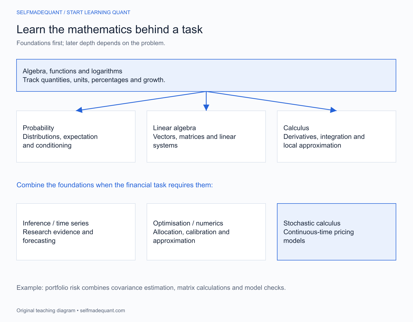
The mathematical toolkit at a glance

Subject	Learn to do	A financial use
Algebra, functions and logs	Rearrange equations and track units	Returns, discount factors and growth
Calculus	Differentiate, integrate and approximate locally	Sensitivities, accumulated cash flows and densities
Linear algebra	Work with vectors, matrices and linear systems	Portfolios, regression and factor exposure
Probability	Model uncertainty and condition on information	Random payoffs, forecasts and stochastic models
Statistics	Estimate, compare and quantify uncertainty	Research evidence and risk estimation
Optimisation	Define an objective and constraints	Allocation, calibration and execution
Numerical methods	Approximate and diagnose error	Pricing, root finding and simulation
Stochastic processes and calculus	Model random evolution through time	Continuous-time derivatives models

These subjects interact. Estimating a covariance matrix involves statistics; using it in a portfolio calculation involves linear algebra; selecting weights can involve optimisation. Understanding all three prevents the optimiser's answer from seeming more certain than its inputs.

1. Algebra, functions and logarithms

Begin with percentages, equations, powers, exponentials, logarithms and function notation. Track the units of each quantity. An annual rate, a daily return and an amount of cash cannot be substituted for each other because their numerical values look similar.

For simple returns $r_1,\ldots,r_T$ , wealth with no external cash flows evolves as:

W_T=W_0\prod_{t=1}^{T}(1+r_t).

Log returns make this multiplicative relationship additive when prices are positive. That is a mathematical convenience, not permission to ignore the difference between a log return and a simple return in reporting.

Start with arithmetic, algebra and functions and exponentials and logarithms. The beginner guide works through a loss-and-recovery example.

2. Calculus: change and local approximation

Differentiation measures local sensitivity. If a model's option value is $V(S)$ , its delta with respect to the underlying price is $dV/dS$ under the stated inputs. A small move can be approximated by:

V(S+\Delta S)\approx V(S)+\frac{dV}{dS}\Delta S.

The approximation is local. A large move can make curvature important. A sensitivity calculated while holding volatility fixed also need not describe a market move in which volatility changes.

Integration connects densities with probabilities and averages, and appears in valuation and accumulated quantities. Multivariable calculus becomes useful when the result depends on several inputs.

Use the primer lessons on differentiation, integration, and partial derivatives. MIT's single-variable calculus course supplies a broader exercise sequence.

3. Linear algebra: portfolios and dependence

A portfolio's weights form a vector. Its estimated return relationships can be represented by a covariance matrix. For weights $w$ and covariance matrix $\Sigma$ , model variance is:

\sigma_p^2=w^\top\Sigma w.

That compact expression contains an economically important idea: dependence changes aggregate risk. Adding assets does not guarantee a large diversification benefit.

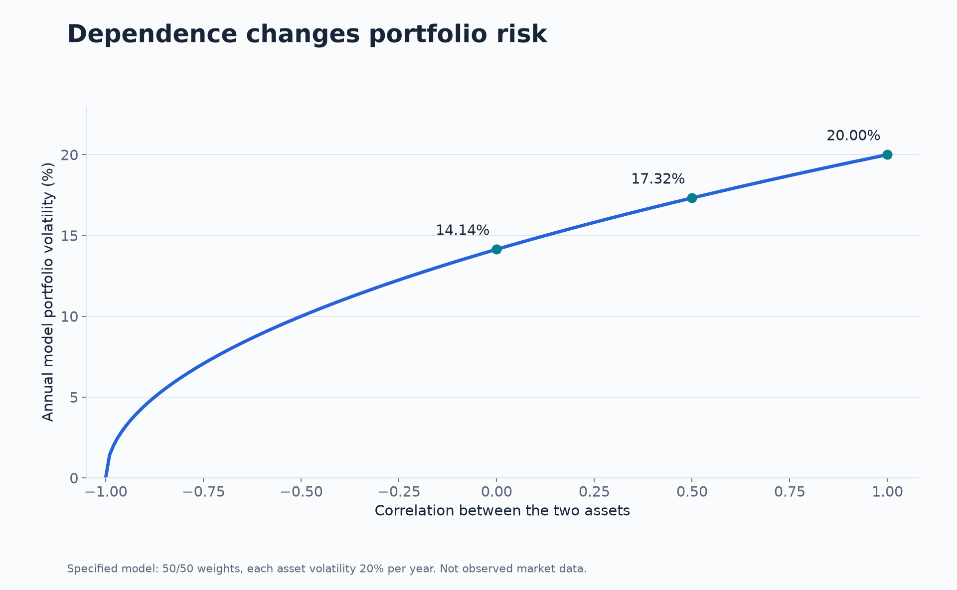
Worked example: two equally volatile assets

Take two assets with annual model volatility 20% each, weights of 50% each and correlation $\rho$ . Assume the covariance model is valid for the horizon and ignore leverage and costs. Then:

\sigma_p^2=0.5^2(0.20)^2+0.5^2(0.20)^2+2(0.5)(0.5)(0.20)(0.20)\rho.

With zero correlation, model volatility is approximately 14.14%. With correlation 0.5, it is approximately 17.32%. With correlation 1, it is 20%: splitting the capital does not reduce volatility in this example.

Annual model volatility of a fifty-fifty portfolio rises with correlation between two assets, each with twenty-percent model volatility.

Specified two-asset model, not observed market data. Correlation and volatility estimates can change; the curve is not a risk forecast.

from math import sqrt

asset_vol = 0.20
for correlation in (0.0, 0.5, 1.0):
    variance = 0.5 * asset_vol**2 * (1.0 + correlation)
    print(f"{correlation:.1f}: {100.0 * sqrt(variance):.2f}%")
# 0.0: 14.14%
# 0.5: 17.32%
# 1.0: 20.00%

Study vectors, matrices and linear systems, then eigenvalues and covariance matrices. Gilbert Strang's MIT course develops the formal toolkit; 3Blue1Brown's series provides a visual companion.

4. Probability: information and uncertainty

Learn random variables, distributions, expectation, variance, independence and conditioning. A probability statement depends on both the model and the information being used.

For example, knowing that at least one of two fair coin flips is heads differs from knowing that the first flip is heads. The possible outcomes remaining after the observation differ. The same discipline matters when you condition a financial forecast on what was actually observable.

Conditional expectation is especially useful later. It leads to martingales, dynamic models and many pricing arguments. Harvard Stat 110 offers a substantial probability foundation with practice and video links.

Where martingales fit

A martingale is an integrable stochastic process whose conditional expected future value equals its current value, relative to a specified information set and probability measure. The information and measure are part of the definition.

In suitable no-arbitrage pricing models, discounted tradable prices are modelled as martingales under a pricing measure. This does not say an actual stock price has zero expected growth under your real-world forecasting model. It also does not endorse the similarly named doubling betting strategy.

Learn conditioning and stochastic processes before memorising martingale statements. The market model and risk-neutral valuation lesson supplies financial context.

5. Statistics: evidence and estimation error

Statistics helps you infer from a finite sample. Learn sampling variation, estimation, confidence intervals, hypothesis testing, regression and validation. Then investigate what changes when observations are dependent or the model was selected after many attempts.

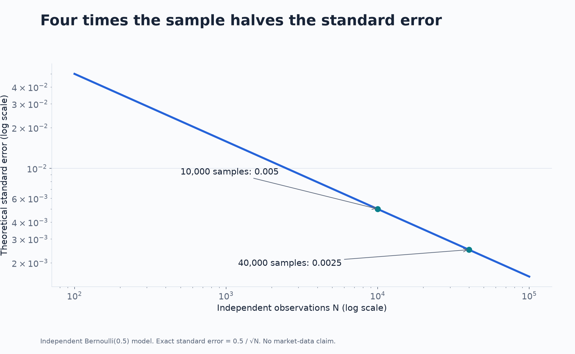
For independent observations with a common finite variance, the standard error of a sample mean scales as $1/\sqrt{N}$ . Multiplying sample size by four halves this standard error. That relationship is useful for simulation, but financial time-series dependence can invalidate a naive independent-observation calculation.

The theoretical standard error of an independent fair-coin payoff mean falls with sample size; four times as many observations halves the standard error.

Exact standard-error formula for independent Bernoulli observations with probability 0.5. This is a sampling model, not an empirical claim about market data.

Use confidence intervals and hypothesis testing, followed by linear regression. StatQuest's video index is a useful supplementary source for focused statistical explanations. Work through exercises as well as watching the explanations.

6. Optimisation and numerical methods

Optimisation begins with an objective and constraints. “Find the best portfolio” is incomplete until you say what best means, what estimates you use, and what positions are permitted. A mathematically optimal solution can be fragile if the inputs are uncertain.

Numerical methods introduce approximations. Learn finite differences, root finding, integration, simulation and convergence checks. Distinguish sampling error, discretisation error, input error and model error; increasing the sample size addresses only some of these.

Use constrained and convex optimisation, numerical differentiation, and the Monte Carlo option-pricing article.

7. Stochastic calculus: when continuous time matters

Brownian motion, stochastic differential equations and Itô's lemma are important in many continuous-time derivatives models. Itô's lemma describes how a sufficiently smooth function of an Itô process evolves, including the second-order contribution associated with quadratic variation.

This is advanced material with prerequisites. An intuitive video can help you see why an ordinary chain rule is insufficient, but you still need probability, calculus and a clear stochastic model to use the result correctly.

Begin with the Brownian motion and Itô's lemma lesson inside Options Pricing. A researcher working on daily empirical forecasts may initially benefit more from statistics and validation than from advanced stochastic calculus. That priority can change with the research problem.

Prioritise by the task you want to perform

First direction	Put early effort into	Add when the work requires it
Empirical research	Probability, statistics, regression, time series	Advanced inference, optimisation and specialised models
Trading and execution	Probability, estimation, instruments, market mechanics	Stochastic control or other strategy-specific mathematics
Pricing	Calculus, probability, numerical methods, replication	Stochastic calculus and richer models
Portfolio and risk	Covariance, inference, optimisation, time series	Tail models, credit models and advanced dependence
Development	Algorithms, numerical reliability and relevant domain maths	Deeper mathematics for the models you implement

The table is a study recommendation. Actual roles can require depth across several rows.

How to check whether you understand enough to move on

For each subject, explain one financial quantity, solve a small example, implement it, and change an assumption. You should be able to identify what breaks.

For linear algebra, change the correlation in the portfolio example. For probability, change the information observed. For numerical methods, change the step size or sample size. For calculus, compare a local approximation with the full function over a larger move.

If the result surprises you, that is a useful place to study. If you cannot say what the output's units are, return to the definition before making the model more complex.

Your next programme

Use the Mathematics Primer for foundation gaps. Continue into Probability, Statistics and Financial Data and Linear Algebra, Optimisation and Numerical Methods. Pair each programme with a small project from the roadmap, so the mathematics has a quantity, decision and check attached to it.

For a worked continuous-time sequence, continue through martingales, Brownian motion and Itô’s lemma. Each page develops one concept and connects it to a checked financial calculation.

Download the accompanying Python examples

Get the series code package. The download contains four runnable beginner examples, an editable notebook and generators for the compounding, portfolio-correlation and Monte Carlo charts. Start with the unchanged examples, then alter one assumption and explain the result. Downloads use the app’s usual email or member access.