Python for quant finance: what to learn first, with a runnable example
Start Python for quant finance with functions, collections, files and error handling. Then learn NumPy arrays, pandas tables and time indexes, plotting, and reproducible numerical experiments. Your first goal is a calculation with explicit inputs, a known benchmark and a useful check. Large models and live trading systems come later.
Python lets you turn a mathematical question into an experiment you can repeat. That is valuable only if you understand the data and the quantity being calculated. A fast function can produce an incorrect answer consistently; reproducibility and correctness are different requirements.
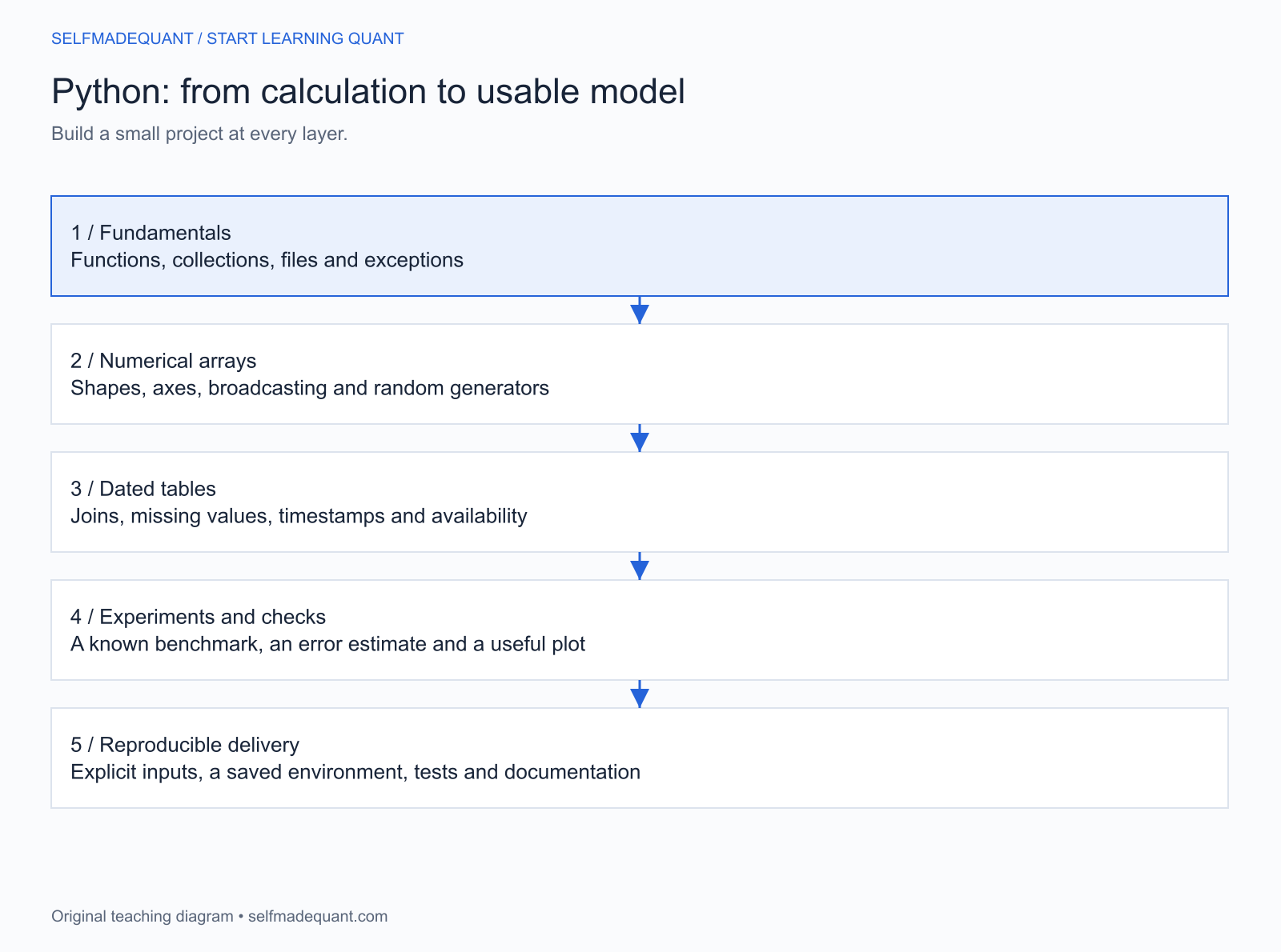
1. Learn enough Python to express the problem
Begin with variables, numeric types, Boolean conditions, loops, functions, lists, dictionaries and file handling. Learn to read an error message and to distinguish an invalid input from a numerical result.
Write small functions before building a large notebook. A function makes the inputs and outputs visible and gives you something you can check independently.
def simple_return(previous_price, current_price):
    if previous_price <= 0.0 or current_price <= 0.0:
        raise ValueError("This example requires positive prices.")
    return current_price / previous_price - 1.0

print(f"{100.0 * simple_return(100.0, 102.0):.2f}%")
# 2.00%
This function deliberately assumes positive prices. It is an introductory calculation, not a complete representation of every financial instrument or corporate action. State that boundary rather than silently treating the function as universal.
2. Learn arrays before optimising everything
NumPy arrays represent numerical collections. Learn shapes, indexing, broadcasting, aggregation and random-number generators. Always check which axis a calculation uses.
A table with observations in rows and assets in columns is different from its transpose. An operation that broadcasts successfully can still implement the wrong financial equation.
Performance work should begin with a measured bottleneck. Replacing readable code with a complicated expression is not progress if you can no longer verify what it calculates.
3. Learn tables, dates and information timing
Financial data usually have identities and timestamps as well as numbers. pandas helps with tables, joins, missing values and time-indexed data, but it cannot decide which timestamp represents availability to a trading decision.
Suppose a company report refers to a quarter ending in March and is released in May. Joining the final reported value onto every day in March creates information your historical experiment could not have known then.
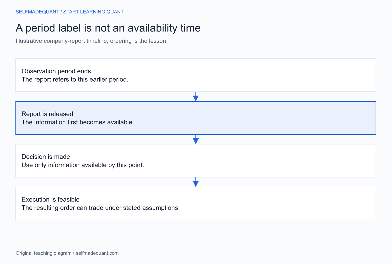
For every dataset, record what a row represents, units, timezone, source, missing-value policy and revision behaviour. A plot alone cannot establish that these choices are correct.
4. Run a small Monte Carlo experiment
Monte Carlo estimates an expectation using random samples from a specified model. Before simulating asset prices, use a payoff with a known answer: 1 if a fair coin lands heads and 0 otherwise.
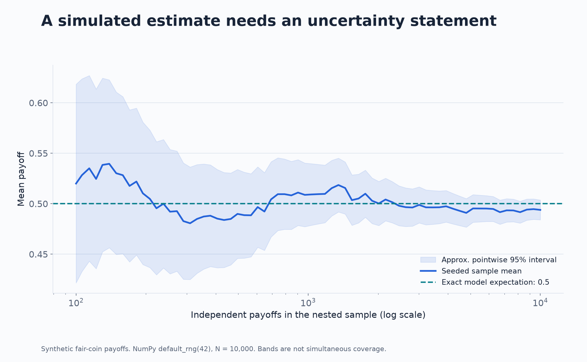
Under the fair-coin model, expected payoff is 0.5. We will generate 10,000 independent observations, estimate their mean and calculate an estimated standard error. This is a synthetic probability experiment, not trading performance.
default_rng with seed 42. The same generator, seed and call sequence make this example repeatable within the documented setup; a seed does not control unrelated data or external systems.import numpy as np
rng = np.random.default_rng(42)
n_samples = 10_000
payoffs = rng.integers(0, 2, size=n_samples)
estimate = float(payoffs.mean())
sample_std = float(payoffs.std(ddof=1))
standard_error = sample_std / np.sqrt(n_samples)
lower = estimate - 1.96 * standard_error
upper = estimate + 1.96 * standard_error
print(f"Mean: {estimate:.4f}")
# Mean: 0.4939
print(f"Estimated standard error: {standard_error:.4f}")
# Estimated standard error: 0.0050
print(f"Approximate 95% interval: [{lower:.4f}, {upper:.4f}]")
# Approximate 95% interval: [0.4841, 0.5037]
print(f"Exact model expectation: {0.5:.4f}")
# Exact model expectation: 0.5000The estimated standard error measures sampling uncertainty in the mean. It is different from the standard deviation of individual payoffs, which is close to 0.5. Confusing the two would make the uncertainty statement about 100 times too wide here.
The interval is a normal approximation for this large independent sample, not a guarantee that an unknown expectation lies inside it. Under repeated sampling, its intended coverage is approximately 95%; the fixed parameter is not being randomly redrawn with each interval.
What should you check?
Confirm that the payoff values are only 0 and 1, that the sample count is correct, and that the known expectation is within a plausible range of the estimate. Do not write a test requiring every simulated interval to contain 0.5: legitimate sampling variation can make that fail.
Check the theoretical standard error under the model:
At 10,000 observations it is 0.005. Increasing the sample count to 40,000 halves this theoretical value. Individual realised errors need not shrink monotonically as you add samples.
How does this connect to option pricing?
An option payoff is another random quantity under a chosen model. A Monte Carlo pricer samples that payoff under the appropriate pricing assumptions, discounts it consistently and estimates uncertainty.
5. Plot results with a question in mind
A useful chart reveals an uncertainty, comparison or failure. Plot a model estimate against its known benchmark, show residuals, or examine sensitivity to a parameter. Label the units and distinguish simulated data from observed data.
For the coin experiment, the useful question is how the estimate and its uncertainty change with sample size. A decorative histogram alone would not answer that question.
6. Make the project reproducible
Keep a notebook for exploration, but move reusable calculations into functions. Record input data and configuration, pin the relevant environment, and make it possible to rerun the result from a clean start.
Add a small number of meaningful checks: a known formula, an accounting identity, a limiting case and an invalid input. A test that simply repeats the implementation is weak evidence.
Choose a first Python project
| Project | What you practise | A strong check |
|---|---|---|
| Return calculator | Functions, arrays and financial units | Compounded returns match the price ratio under stated assumptions |
| Coin-payoff simulation | Random generators and sampling error | Compare with a known expectation and theoretical standard error |
| Portfolio-risk calculator | Matrix operations and covariance | Check a one-asset or perfectly correlated limiting case |
| European option pricer | Functions, model inputs and numerical comparisons | Compare with an independent formula or method |
| Dated decision ledger | Tables, joins and information timing | Trace one decision using only available observations |
Common questions
Is Python enough for quant finance?
Should I learn machine learning before pandas?
Learn the data operations needed to build a valid experiment first. A complex estimator cannot fix a forward-looking join, duplicated observation or incorrect target. Begin with a baseline you can inspect.
Do I need market data for my first project?
No. Synthetic data and small illustrative fixtures let you check the calculation against known quantities. When you introduce market data, document sourcing, adjustments, timing and limitations rather than assuming the dataset is ready for research.
Continue with a structured programme
Download the accompanying Python examples
Go deeper with lessons, derivations and worked exercises behind this article.