A volatility forecasting project in Python: four models, one clock and an honest risk report
A volatility project should produce more than a smooth line over a chart. Another person should be able to rerun it, identify what the model knew before each observation and understand which result would change if an assumption failed.
This final article assembles that workflow. The project runs with the Python standard library and writes the data, forecasts, risk thresholds and numerical checks to local files. It uses a seeded synthetic sample so the experiment is reproducible without a data subscription.
Synthetic data give us control over the mechanism. They do not establish that a model works on an exchange or that a risk policy can be traded profitably.
Know how the sample was constructed
The generator produces 1,500 decimal-return observations after a 500-observation burn-in. Its initial variance recursion has ω = 0.000002, α = 0.08 and β = 0.90. Innovations follow a symmetric Student-t distribution with seven degrees of freedom, scaled to variance one.
The seed is 20261014. After the return at session 1000, the generator changes ω to 0.000008. That creates a persistent change in the variance level. The forecasting models are not given that event as a feature.
We save the latent conditional variance because the simulator knows it. It is used only for a labelled diagnostic after the forecast choices have been made. A real closing-return dataset would not provide that column.
These choices make the sample a controlled challenge: heavy tails, volatility persistence and an unexpected level change. They do not describe every market or guarantee that the same ranking would appear on another seed.
Freeze the research boundary
Use the first 600 observations for initial fitting, the next 300 for validation and the final 600 for evaluation. The candidate lists are fixed in the source.
Validation compares four EWMA decay values and three rolling-window lengths. It selects decay 0.90 and a twenty-observation window. The final GARCH fit uses the first 900 observations once, then holds its parameters fixed through evaluation.
The GARCH estimator evaluates sixty feasible candidates with a Gaussian quasi-score. It is a coarse grid, not a continuous optimum. Its selected persistence is 0.985, the upper edge of the declared persistence grid. That is a limitation worth recording rather than a convergence result to celebrate.
Model states still update after each new return. This is permitted information flow. The final observations do not select the decay, the rolling window or the GARCH parameters.
Make the forecast before consuming its target
For every final observation, save the forecast origin as the preceding session. The EWMA and GARCH loops append the current variance before updating it with the newly observed return.
def garch_forecasts(returns, omega, alpha, beta, initial):
    variance = initial
    forecasts = []
    for observed_return in returns:
        forecasts.append(variance)
        variance = omega + alpha * observed_return**2 + beta * variance
    return forecasts

print(garch_forecasts([-0.03], 0.000002, 0.08, 0.90, 0.0001))
# [0.0001]
The next state after that return is 0.000164. Using that next state as the forecast for the same observed return would give the model information it did not have in advance.
The project checks this beyond a visual inspection. Removing observations after a cutoff leaves all earlier final forecasts unchanged. Replacing those future returns with extreme values also leaves the earlier forecasts unchanged. These checks would catch several common alignment mistakes.
They do not prove the entire research process is free of leakage. The split protocol, fit endpoints and parameter selection also need inspection.
Compare four explicit forecasts
The fixed baseline uses the fit sample's second moment. The rolling forecast averages recent squared returns. EWMA applies its selected decay recursively. GARCH uses its frozen fitted coefficients and an updating variance state.
All forecasts target one-session, zero-mean variance in decimal-return units. The main evaluation score is log(h) + R²/h. We also save variance MSE and a separately labelled latent-variance diagnostic.
| Forecast | Final mean score | Gaussian 99% VaR breaches |
|---|---|---|
| Fixed second moment | −4.700897 | 60 |
| Rolling twenty observations | −7.094087 | 11 |
| EWMA, decay 0.90 | −7.113430 | 12 |
| Frozen GARCH grid | −7.108327 | 11 |
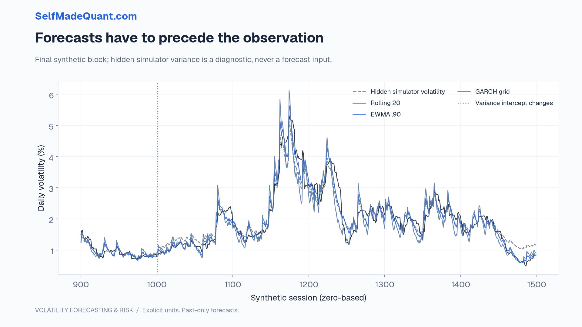
EWMA has the lowest main score on this path. GARCH and rolling are close. The fixed baseline responds poorly to the later variance level because it never updates.
The relative model ranking is not a statistical significance result. We do not search another seed because the first result is inconvenient, and we do not retune parameters on these final scores.
Build the risk report without inventing a trading strategy
For each GARCH forecast, the output includes Gaussian 99% VaR and ES in return units. Multiplying by an appropriate fixed linear exposure converts them into dollar thresholds under the stated assumptions.
The output also includes exposure for a 10% annualised volatility target, capped at 1.5 times capital. This is a sizing snapshot. The dataset contains no separate opening prices, executable quotes, borrowing conditions or order fills.
We therefore report no trading return, Sharpe ratio or transaction-cost-adjusted profit for the exposure rule. Those claims would require a feasible execution timeline and a portfolio ledger that this experiment does not provide.
The VaR exceptions also reveal a modelling limitation: Gaussian thresholds are being applied to heavy-tailed innovations. Eleven or twelve breaches in 600 observations exceed the nominal six expected under a correctly calibrated 1% rate, but the project does not convert that comparison into an unreported formal test. ES forecasts are provided for inspection, not certified by the VaR count.
Reproduce and inspect the files
python3 lab/volatility_risk_lab.py from the campaign folder. The script overwrites its deterministic outputs: synthetic_returns.csv, final_forecasts.csv and results.json.The results record the seed, split boundaries, selected candidates, scores, checks and limitations. The forecast CSV retains both the target session and forecast origin. The separate figure script reads those files to build the illustrations; it does not alter the numerical experiment.
A useful extension is to run the frozen design across several prespecified seeds and report the distribution of score differences. Another is to replace the synthetic sample with properly documented market data, then reconsider the measurement target, cleaning policy and execution assumptions.
Neither extension should quietly reuse the current final block as though it were new evidence. Keep a research log and label the next experiment honestly.
The series began with a question about the meaning of one volatility number. It ends with a reproducible report in which the units, information set, forecast target and limits of the conclusion are visible. That is the foundation for a model another person can trust enough to challenge.
Until then, peace.
Go deeper with lessons, derivations and worked exercises behind this article.