Asymmetric volatility and heavy tails: two different ways a risk model can miss the loss

A +3% return and a −3% return have the same square. In the simple GARCH model, they therefore produce the same next variance forecast when everything else is held fixed.

That symmetry is a modelling restriction. We can relax it. Separately, we can change the distribution of the standardised shock so that extreme observations occur more often than a Gaussian model expects.

These are two different changes. An asymmetric variance update describes how past information changes future scale. Heavy-tailed innovations describe the shape of returns after accounting for that scale.

Give negative shocks a different coefficient

A GJR-style variance equation adds an indicator for a negative residual:

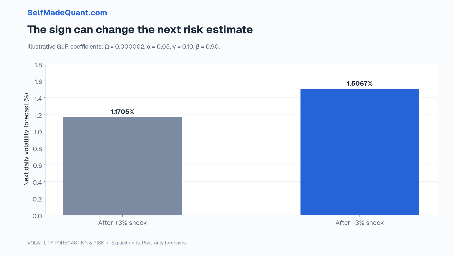
For this example, set ω = 0.000002, α = 0.05, γ = 0.10 and β = 0.90. Start with variance 0.0001.

A +3% shock gives a next variance of 0.000137, or approximately 1.1705% daily volatility. A −3% shock gives 0.000227, or approximately 1.5067% daily volatility.

The extra γ term changes the reaction to the negative shock. It does not mean that every market, instrument or historical period has this response. It does not establish an economic explanation for an estimated asymmetry either.

Under symmetric variance-one innovations, the expected negative-shock squared term is half the total second moment. The familiar finite-variance condition then involves α + β + γ/2. With a different innovation distribution, use the actual expected value of Z² times its negative-side indicator; the one-half shortcut may fail.

A fat tail is not a time-varying variance

Imagine standardising a return by its forecast scale: Zₜ = εₜ/√hₜ. If the scale model works well, large predictable changes in variance should no longer dominate the standardised sequence.

That sequence can still have more extreme observations than a standard normal distribution. A Student-t innovation distribution is one way to represent that feature.

A conventional Student-t random variable with ν degrees of freedom has variance ν/(ν − 2) when ν > 2. To use it as a variance-one innovation, multiply it by √((ν − 2)/ν).

With seven degrees of freedom, the multiplier is √(5/7). Omitting this scaling makes hₜ a scale parameter rather than the conditional variance described by our equations. The simulation can run perfectly while the model's labels become wrong.

At ν ≤ 2, the usual variance does not exist. Between two and four degrees of freedom the variance exists but the fourth moment does not. The choice affects which moment-based diagnostics and uncertainty calculations are well behaved.

Our project uses variance-one Student-t innovations with seven degrees of freedom. The heavy tails are part of the simulator design, not a distribution fitted to actual market data.

Scale and tail shape need separate checks

Suppose your variance forecast matches the true conditional variance. You then use a standard normal 99% quantile to turn that scale into a loss threshold.

If the actual standardised shocks are heavy-tailed, the threshold can still be breached too often. Improving the variance recursion alone may not solve the calibration problem.

Conversely, replacing a normal distribution with a Student-t distribution does not repair look-ahead bias, a poor conditional mean or an incorrect timestamp. It cannot make a stale variance estimate timely.

Inspect standardised residuals for serial correlation and squared-residual dependence. Examine tail quantiles and exceedance patterns. If there is remaining time structure in the squared residuals, the variance model may have left predictable variation behind. If their scale is stable but the tails are wrong, the distributional assumption deserves attention.

Neither diagnostic is a proof based on one chart. Small samples, fitted parameters and model selection all affect interpretation. A residual plot should generate questions rather than certify the model.

Add complexity only when its job is clear

An asymmetric recursion can improve fit while adding estimation uncertainty. A heavy-tailed distribution can absorb extreme observations while changing the likelihood surface and tail estimates. Combining both increases the number of decisions made before evaluation.

Write down the comparison before looking at the final sample: symmetric versus asymmetric variance, normal versus variance-standardised Student-t innovations, the same information set and the same forecast target.

Keep a simple benchmark. If a more elaborate model improves a fitted likelihood but does not improve later variance scores or risk calibration, explain that outcome. It may be useful for one task and unnecessary for another.

The accompanying project keeps the final forecast comparison deliberately small. Its GARCH fit uses a Gaussian quasi-score even though the innovations are heavy-tailed. The resulting Gaussian loss thresholds are then tested openly rather than labelled calibrated by construction.

The aim is to learn which component caused a failure. Was the forecast scale stale? Did the tail assumption understate extreme shocks? Did an observation arrive too late to be used? Those explanations lead to different repairs.

Next, we will choose a scoring rule and see why “closest to tomorrow's squared return” is an incomplete description of a good variance forecast.

Until then, peace.