Value at Risk and Expected Shortfall: a threshold is not a maximum loss

A report gives a one-day 99% Value at Risk of 23,263 on a position worth one million. Does that mean the position cannot lose more than 23,263 tomorrow?

No. It is a quantile of a specified loss distribution. It needs a horizon, a confidence level, an information set and a sign convention. Outcomes beyond the threshold are part of the distribution, not a contradiction of its definition.

Expected Shortfall asks a related question about the severe-loss tail. Understanding the difference is useful before you connect either measure to a limit.

Define losses with the positive sign

For a fixed, unleveraged long position with initial value V and simple return R, write loss as L = −VR. A negative return produces a positive loss.

This is exact for that linear position over the specified holding interval. An option portfolio, a changing position or a return expressed in log units needs a different mapping or a stated approximation.

At confidence c, define:

This left-quantile definition matters for discrete samples. Different interpolation rules can produce different reported sample quantiles, particularly when the sample is small.

If the distribution is continuous, a correctly calibrated 99% threshold has a 1% probability of being exceeded under the stated information set. For distributions with atoms, the exceedance probability can be smaller because probability mass can sit exactly at the quantile.

Work through the Gaussian example

Assume zero mean, one-day return volatility of 1% and a Gaussian return distribution. A one-million position then has a loss standard deviation of 10,000.

The 99% standard normal quantile is approximately 2.32635. The VaR is therefore approximately 23,263.48.

For a Gaussian loss distribution with mean μ and standard deviation σ:

At the same confidence level, zero mean and 10,000 standard deviation, Expected Shortfall is approximately 26,652.14. The tail average exceeds the boundary of the tail.

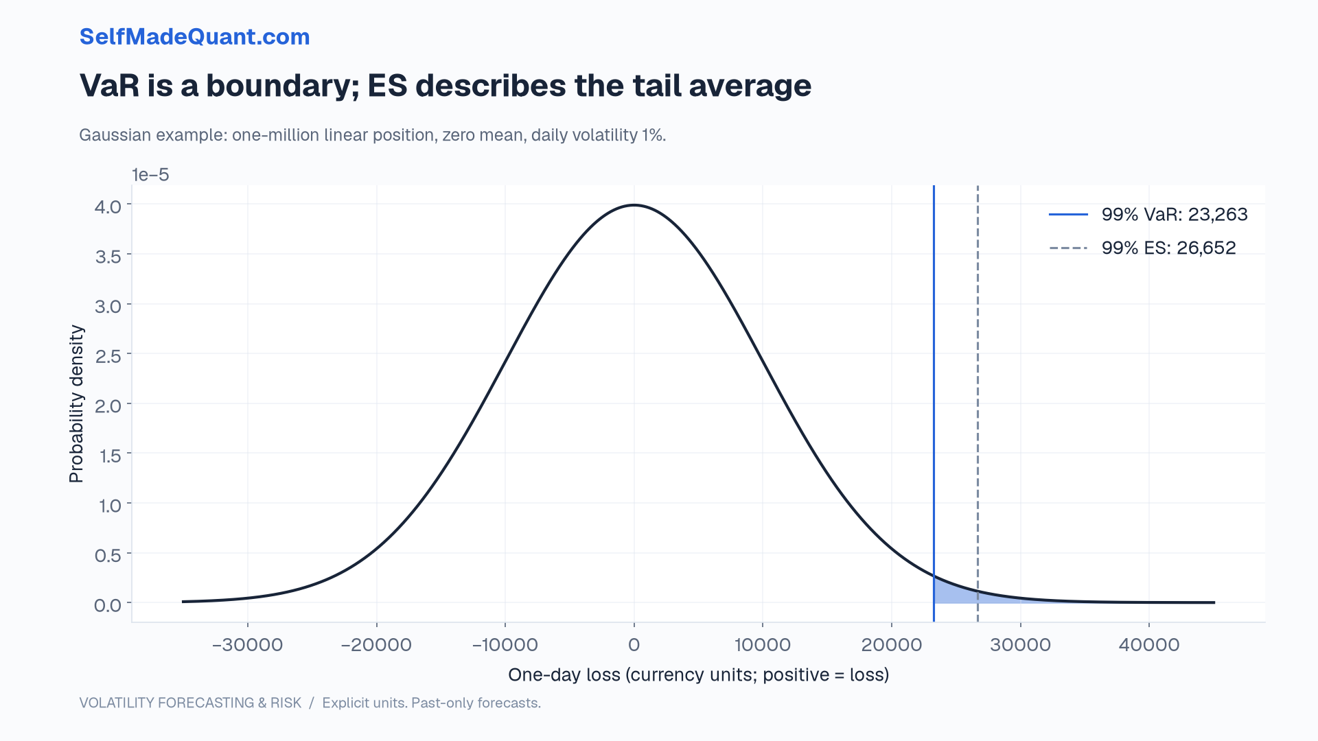
Every number depends on the distributional assumption. Replacing the Gaussian shocks with variance-standardised Student-t shocks changes the tail calculation even when the volatility forecast stays at 1%.

The discrete-tail trap

A useful general definition is:

assuming the required integrability. This handles probability mass at the quantile without pretending that every discrete tail is a continuous one.

Consider losses of zero with probability 98%, ten with probability 1%, and one hundred with probability 1%. The 99% VaR is ten. The worst 1% of outcomes are all the hundred-loss state, so 99% ES is one hundred.

Taking the average conditional on L ≥ ten instead gives fifty-five. That includes 2% of the probability mass, which is the wrong tail size for this confidence level.

For an empirical sample, use a documented quantile convention and fractional weighting at the boundary when the desired tail mass falls inside an observation's probability weight. A simple average of every observation at or above an interpolated quantile is not a universal ES estimator.

Count breaches, then inspect their timing

Our project calculates Gaussian 99% VaR from each variance forecast, then compares it with the next synthetic loss. The simulator uses heavy-tailed shocks, so Gaussian tail calibration is an assumption being tested.

Over the 600 final observations, the fixed baseline has sixty breaches, the rolling forecast eleven, EWMA twelve and the GARCH grid eleven. A nominal 1% rate corresponds to six expected breaches, not an entitlement to exactly six in every sample.

Counts alone leave out timing. Eleven breaches scattered through the sample and eleven clustered in a short stressful episode are different diagnostic patterns. Plot the exception dates alongside the forecast scale and investigate what information the model missed.

Do not infer a formal rejection from a count without specifying a test. A binomial calculation assumes an appropriate independent Bernoulli structure; conditional coverage questions also examine dependence. Parameter estimation and repeated model selection can complicate the interpretation further.

Expected Shortfall needs its own evaluation

A VaR exception count does not validate ES. The model might predict the frequency of extreme losses reasonably while badly understating their severity.

ES assessment needs information about the tail losses and the accompanying quantile forecasts. A serious evaluation should specify a suitable joint scoring or backtesting approach, its assumptions and its sample limitations. With 600 observations at a 99% confidence level, the nominal tail contains only about six observations on average; severe-loss inference is necessarily fragile.

The lab reports Gaussian ES forecasts for inspection but does not claim that its breach count validates them. That distinction should survive the journey from notebook to presentation.

A limit is a policy layered over a model

A loss measure can inform a position limit, but it does not implement one. The policy must define what happens when the limit is exceeded, how quickly positions can change and how gaps, funding and execution costs are handled.

Next, we will see why calculating each asset's volatility separately is insufficient for a portfolio. The interaction between positions can change the loss distribution before any individual estimate moves.

Until then, peace.