How to evaluate volatility forecasts: QLIKE, noisy targets and an untouched final sample
Two variance forecasts disagree. One is smoother. The other reacts quickly to yesterday's shock. Which one is better?
A chart is not enough. You need to specify the quantity being forecast, the later observation used to judge it and the score that connects them. Then you need a sample that was not used to choose the model.
In volatility forecasting, the evaluation target itself is often noisy. That makes the scoring decision part of the research design rather than a cosmetic choice at the end.
Start with an honest proxy
Let hₜ be a forecast made before return Rₜ arrives. Under a correctly specified zero conditional mean, Rₜ² is conditionally unbiased for the return variance.
It is also a noisy observation. A near-zero return does not establish that the day's conditional variance was near zero. A very large return does not establish that a high variance forecast should have been known in advance.
If the conditional mean is nonzero, the raw squared return estimates a second moment. You need an appropriately defined residual or a target that explicitly includes the mean term. Subtracting a mean estimated with future data introduces a different problem.
An intraday realised-variance proxy may offer more information, but it brings the sampling and measurement questions from the earlier article. Choose the proxy before comparing model rankings.
Squared error answers one question
The variance mean-squared error uses (yₜ − hₜ)², where yₜ is the chosen variance proxy.
It penalises large absolute errors strongly. Its units are squared variance units, so rescaling decimal returns into percentage points changes its numerical magnitude dramatically. Rankings survive a consistent common rescaling, but a raw score cannot be compared across inconsistent unit conventions.
A quasi-likelihood score works on positive variance forecasts
Our project uses:
Lower is better. For a positive proxy y, this has the same model ranking as the normalised QLIKE expression y/h − log(y/h) − 1. They differ by terms depending on y alone, which cancel when comparing forecasts on the same observations.
Unlike the normalised expression, log(h) + y/h can be negative. That is not an error. Its absolute level depends on the variance units, and comparisons require the same target observations.
It also remains defined when y is zero, provided h is positive. We impose a tiny documented numerical floor on forecasts to prevent division by zero. A floor that frequently activates is a model diagnostic; it should not become an undisclosed way to rescue failed forecasts.
Consider y = 0.0001. A matching forecast h = 0.0001 has normalised QLIKE zero. Forecasting half that variance gives approximately 0.30685; forecasting twice it gives approximately 0.19315. Relative underprediction and overprediction receive different penalties.
The derivative of the expected log-plus-ratio score with respect to h is (h − E[y|information])/h². Under a conditionally unbiased proxy, its optimum is the conditional variance. This calculation explains the score's target in our setup.
Separate selection from evaluation
Our synthetic experiment has 1,500 observations:
- Sessions 0–599: initial fitting.
- Sessions 600–899: validation of EWMA decay and rolling-window length.
- Sessions 900–1499: final evaluation.
The candidate grids are written in the source before the run. Validation chooses EWMA decay 0.90 and a twenty-session rolling window. Before the final block starts, the GARCH grid is refitted once using the first 900 observations. Its parameters then stay frozen, although its variance state updates as new returns arrive.
Updating a state with yesterday's observation is part of forecasting. Re-selecting a decay parameter after examining final scores is a new research iteration. If you do that, the old final block has become development data.
Read the result at the right strength
On the 600-observation final sample, the mean log-plus-ratio scores are:
| Forecast | Mean score; lower is better |
|---|---|
| Fixed training second moment | −4.700897 |
| Twenty-session rolling second moment | −7.094087 |
| EWMA, decay 0.90 | −7.113430 |
| Frozen GARCH grid fit | −7.108327 |
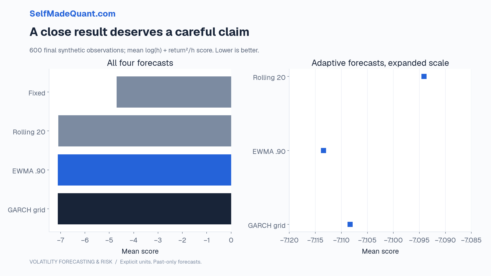
EWMA wins this particular score on this particular path. The difference from the GARCH grid is approximately 0.00510. We do not attach a significance claim or describe it as an economically meaningful market improvement.
The data-generating process contains heavy-tailed shocks and a later variance-level change. The fixed baseline is deliberately slow to adapt. The GARCH search is coarse. Those design choices explain why the result is an experiment about methods rather than a universal leaderboard.
Keep dependence in the uncertainty calculation
Daily score differences can be serially dependent. Overlapping multi-day forecasts create additional dependence because adjacent targets share observations.
A comparison that treats every score difference as an independent draw can understate uncertainty. A more developed study could use a suitable heteroskedasticity-and-autocorrelation-consistent calculation or a carefully designed block bootstrap. The resampling procedure needs to preserve the relevant temporal structure and the selection protocol.
Repeatedly searching models also changes the strength of the final claim. Report the candidate set, unsuccessful runs and any revisions prompted by the evaluation. An apparently untouched date range is not untouched if its results have already guided the research.
Forecast accuracy is only one part of the risk workflow. Next, we will turn a forecast distribution into a loss quantile and a tail-average measure, then ask what their breaches tell us.
Until then, peace.
Go deeper with lessons, derivations and worked exercises behind this article.