Portfolio volatility: the correlation assumption can change the risk budget

Published 14 October 20264 min readVolatility forecasting and risk:Part 1 Part 2 Part 3 Part 4 Part 5 Part 6 Part 7Part 8Part 9 Part 10

You allocate 60% of capital to an asset with 20% annualised volatility and 40% to one with 30%. Is portfolio volatility 24%?

That weighted sum is one particular dependence case. To calculate portfolio variance, you also need the covariance between the returns. Two assets that are individually well measured can still produce a poorly measured portfolio if the interaction is wrong.

This is where volatility forecasting connects directly to portfolio construction. The forecast object becomes a covariance matrix, and the risk budget depends on both the position weights and the estimated relationships.

Calculate the two-asset portfolio

With weights w₁ and w₂, volatilities σ₁ and σ₂, and correlation ρ:

\sigma_p^2=w_1^2\sigma_1^2+w_2^2\sigma_2^2 +2w_1w_2\rho\sigma_1\sigma_2.

For correlation 0.1, the covariance is 0.006. Portfolio variance is 0.03168 and portfolio volatility is approximately 17.80% annualised.

Raise correlation to 0.8 while keeping the same weights and individual volatilities. Portfolio volatility rises to approximately 22.77%. At correlation one it reaches 24%, the weighted sum from the opening question.

These are scenarios under a fixed covariance model. They do not claim that a particular market's correlation will rise to 0.8 during every stress event.

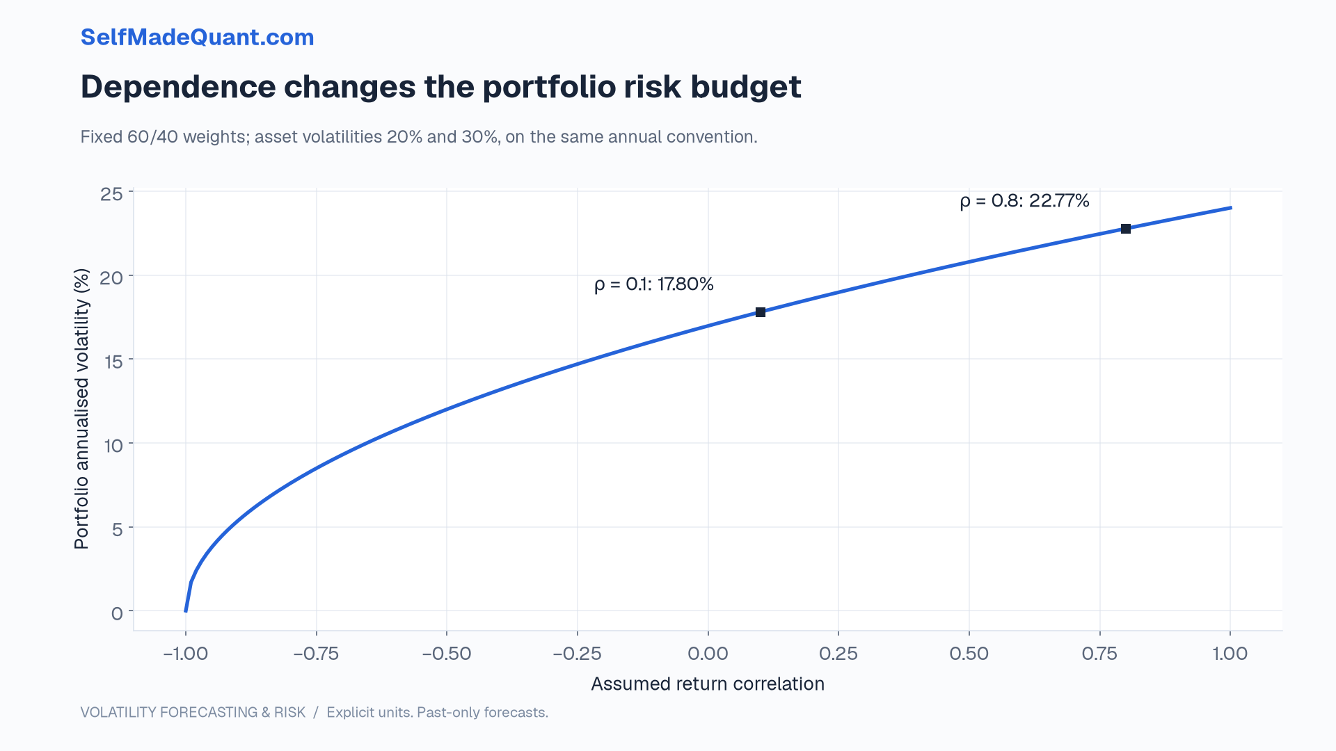
The same weights and asset volatilities produce different portfolio risk as correlation changes

The change has a direct capital implication. A risk limit calibrated using 17.80% cannot be assumed to accommodate a 22.77% scenario without adjustment. The individual-asset volatility cells can remain unchanged while the portfolio breaches its intended budget.

Keep the matrix economically aligned

For many assets, write portfolio variance as wᵀΣw. The row and column labels of Σ must match the ordering of the weights. The return horizon, currency convention and availability time must agree across the inputs.

An array multiplication can succeed with the wrong labels. Combining an annualised covariance matrix with a daily risk target can also produce a finite number. Neither numerical success establishes an economically meaningful calculation.

The matrix should be positive semidefinite so that every portfolio has nonnegative model variance. Pairwise correlations estimated on different missing-data subsets can create an inconsistent matrix even when each individual correlation lies between minus one and one.

A repair or shrinkage method changes the forecast. Record it, compare its consequences and explain the target towards which estimates are being pulled. Do not describe a numerical projection as if it were new market evidence.

Allocate volatility contributions carefully

For a positive portfolio standard deviation, the marginal change with respect to weight i is (Σw)ᵢ/σₚ. Multiplying by the weight gives the Euler contribution:

RC_i=\frac{w_i(\Sigma w)_i}{\sigma_p}, \qquad \sum_i RC_i=\sigma_p.

In the 60/40 example at correlation 0.1, each asset contributes approximately 8.899 percentage points to the 17.799% portfolio volatility. Capital weights differ, yet these two volatility contributions happen to be equal.

That equality comes from the specified numbers. It is not a general property of a 60/40 allocation, and it would change if the covariance estimate changed.

With hedging or short positions, some Euler contributions can be negative. A negative contribution means a local reduction in this model's total volatility; it does not mean the holding has no standalone loss risk or no liquidity requirement.

A volatility target can increase exposure at the wrong moment

Suppose a single-asset policy aims for 10% annualised volatility by setting exposure equal to target divided by forecast volatility.

At a 10% forecast, exposure is one times capital. At a 5% forecast, it becomes two times capital. A leverage cap of 1.5 limits the second decision, but the rule still increases exposure after low estimated volatility.

If a 10% adverse return follows while exposure is 1.5, the approximate linear loss is 15% of capital before execution and financing costs. A historical period of calm did not guarantee a gentle exit.

The forecast is known at a particular timestamp. An actual strategy must specify when the new exposure can be traded and at what price. A close-to-close return series alone does not justify assuming that a decision using the completed close was filled at that same close.

Our lab therefore reports a capped target exposure as a risk snapshot, not a tradable strategy return. This prevents a useful sizing calculation from silently acquiring an infeasible execution assumption.

Evaluate the decision alongside the forecast

Two variance forecasts can produce similar average scores but different turnover and leverage paths. Small forecast changes may cross a policy threshold and generate a large trade. A smoother forecast may reduce trading while responding too slowly after a shock.

If you evaluate a trading policy, keep its costs, timing, cap, financing and execution assumptions explicit. Compare achieved risk, drawdowns, exposure and turnover with a simple baseline. Do not assume the forecast leaderboard determines the policy leaderboard.

Covariance forecasts also need scenarios beyond their central estimates. Test concentrated factors, basis changes, currency moves and weaker hedge relationships. A common dependence model should not be the only story the portfolio report can tell.

Next, we will build a scenario report that keeps probabilities, loss thresholds and funding requirements distinct.

Continue to stress testing. For the allocation background, study mean-variance optimisation.

Subscribe for the series and practise quant interviews.

Until then, peace.