Python interview questions for quants: data, simulation and numerical checks

Published 15 October 20268 min readQuant interview practice:Part 1 Part 2 Part 3 Part 4 Part 5Part 6Part 7

Python interview questions for quants can test financial accounting, time-indexed data, efficient numerical operations, simulation and debugging. A strong solution states the input contract, implements the correct calculation, checks a small case and explains its complexity. Fast code using unavailable information or the wrong financial equation is still wrong.

The five problems below have runnable solutions. They use Python's standard library, with NumPy for the numerical examples. All random examples use a fixed generator seed. The fixtures are illustrative rather than market data, and the questions are not attributed to employers.

If Python itself is new, begin with Python for quant finance: what to learn first. For the wider interview context, use the worked-question overview.

Question 1: calculate total return correctly

Question. Prices are

[100,110,99]

. Write a function calculating the total simple return for a single asset held throughout, with no cash flows or costs. Explain why adding one-period simple returns gives a different answer.

Hint. Check your result against the first-to-last price ratio.

Solution. The period returns are 10% and −10%. Their sum is zero, but compounding gives

1.1\times0.9-1=-0.01

. Under the stated holding assumptions, the same result is

99/100-1=-0.01

The function below requires at least two finite positive prices. That is an explicit input contract for this example, not a claim that every financial instrument always has positive prices.

from math import isfinite

def total_simple_return(prices: list[float]) -> float:
    """Return the buy-and-hold simple return for positive finite prices."""
    if len(prices) < 2:
        raise ValueError("At least two prices are required.")
    if any(not isfinite(p) or p <= 0.0 for p in prices):
        raise ValueError("Prices must be finite and positive.")
    return prices[-1] / prices[0] - 1.0

prices = [100.0, 110.0, 99.0]
period_returns = [current / previous - 1.0
                  for previous, current in zip(prices, prices[1:])]
print(", ".join(f"{100*r:.2f}%" for r in period_returns))
# 10.00%, -10.00%
print(f"Total: {100*total_simple_return(prices):.2f}%")
# Total: -1.00%

Common mistake. Fixing implementation details while leaving the wrong quantity—an arithmetic sum of simple returns—in place. Also check whether a price series includes the adjustments needed for the financial interpretation.

Follow-up. If there are deposits, withdrawals, distributions or changing positions, first-to-last price alone no longer describes the whole investor's wealth calculation. Define the required return measure and cash-flow treatment before extending the function.

Use exponentials and logarithms and testing numerical code. The accounting identity is an independent check, not another copy of an arbitrary loop.

Question 2: use only released information

Question. A value of 10 is released at time 2 and a value of 20 at time 5. For decision times

[1,2,4,5,6]

, return the latest released value available at or before each decision. Return None if nothing has been released. Assume release times are unique, sorted and measured on a common clock.

Hint. A search result before the first release must not index the last element of the list.

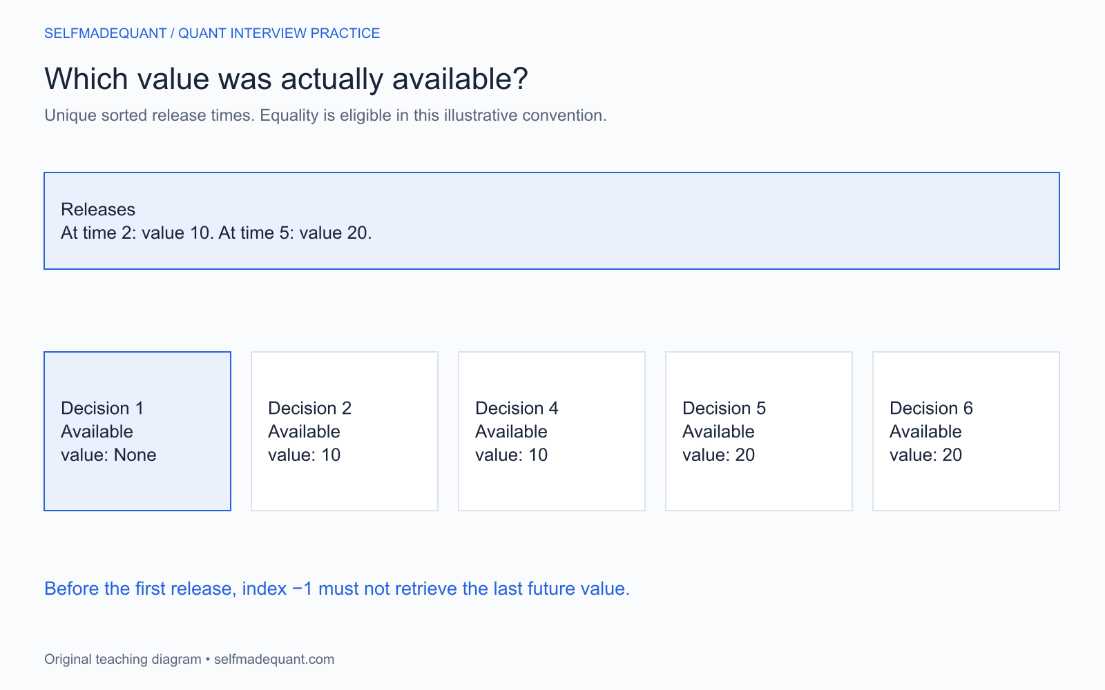
Solution. The answers are

[\text{None},10,10,20,20]

. Binary search identifies the insertion point after all releases with time less than or equal to the decision time. The preceding element, if any, is the latest eligible release.

from bisect import bisect_right

def latest_released(times: list[int], values: list[float],
                    decisions: list[int]) -> list[float | None]:
    """Use the latest unique release with timestamp <= each decision."""
    if len(times) != len(values):
        raise ValueError("Release times and values must align.")
    if any(left >= right for left, right in zip(times, times[1:])):
        raise ValueError("Release times must be strictly increasing.")
    output = []
    for decision in decisions:
        index = bisect_right(times, decision) - 1
        output.append(None if index < 0 else values[index])
    return output

print(latest_released([2, 5], [10.0, 20.0], [1, 2, 4, 5, 6]))
# [None, 10.0, 10.0, 20.0, 20.0]

Validation costs

O(n)

for

n

releases;

m

independent decision searches cost

O(m\log n)

after that, with

O(m)

output space. The searches do not insert into the release list. Python's bisect documentation distinguishes logarithmic searching from linear-time insertion.

A release-time example maps decisions before and after times two and five to only the values available by each decision.

Illustrative integer timestamps. Equality is eligible by the problem's explicit convention; operational event order may require a stricter rule.

Common mistake. Returning values[-1] when the computed index is −1. That supplies the latest future value before any release. A join on a period label can create the same kind of hindsight.

Follow-up. If timestamps have only coarse resolution and releases and decisions share a displayed time, what should happen? Define event ordering or use more precise timestamps. The <= convention here is a modelling choice, not proof that a real order could observe a simultaneously labelled release.

Read observation, event and availability timestamps and tabular and time-indexed data.

Question 3: compute a trailing mean in one pass

Question. For values

[1,2,3,4,5]

, calculate a trailing mean with window three, returning None before a full window exists. Design the calculation to avoid repeatedly summing the whole window. Reject nonfinite values for this version.

Hint. Retain the current sum and remove the oldest value when it leaves the window.

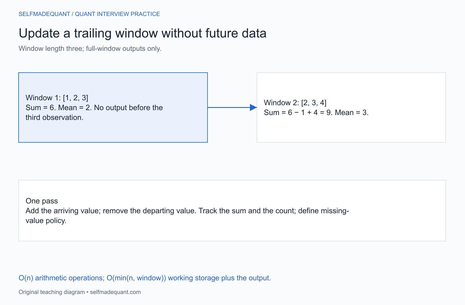
Solution. The complete windows are

[1,2,3]

[2,3,4]

and

[3,4,5]

, with means 2, 3 and 4. A deque lets us append the new value and remove the oldest while updating the sum.

from collections import deque
from math import isfinite

def trailing_mean(values: list[float], window: int) -> list[float | None]:
    """Calculate full-window trailing means for finite inputs."""
    if not isinstance(window, int) or isinstance(window, bool) or window < 1:
        raise ValueError("Window must be a positive integer.")
    queue = deque()
    running_sum = 0.0
    output = []
    for value in values:
        if not isfinite(value):
            raise ValueError("Missing or nonfinite values need an explicit policy.")
        queue.append(value)
        running_sum += value
        if len(queue) > window:
            running_sum -= queue.popleft()
        output.append(running_sum / window if len(queue) == window else None)
    return output

print(trailing_mean([1.0, 2.0, 3.0, 4.0, 5.0], 3))
# [None, None, 2.0, 3.0, 4.0]

Each value is added once and removed at most once: $O(n)$ arithmetic operations, with $O(\min(n,w))$ working storage for window $w$ , plus $O(n)$ output storage. Floating-point accumulation can drift over long or poorly scaled sequences; constant operation count does not eliminate numerical error.

A trailing three-observation window moves from one-two-three to two-three-four, removing one and adding four to update the sum.

Full-window output begins at the third observation. This example rejects nonfinite values instead of silently changing the denominator.

Common mistake. Including future observations in a centred window when the feature is supposed to be available now. Another is treating a window of three observations as three calendar days despite gaps in the timestamps.

Follow-up. How would you handle missing values? Choose a policy—reject, propagate, or average valid values with a minimum count—and track the denominator accordingly. Different policies calculate different statistics.

Use Python's deque documentation, time-series data, and profiling and optimisation.

Question 4: simulate an expectation and quantify error

Question. Estimate the mean of a fair six-sided die using 20,000 independent simulated rolls. Use a fixed seed, report the Monte Carlo standard error and compare with the exact mean 3.5.

Hint. The standard deviation of a roll and the standard error of the estimated mean are different quantities.

Solution. Generate the independent rolls from the stated discrete distribution, then divide their sample standard deviation by the square root of the roll count.

import numpy as np

rng = np.random.default_rng(42)
rolls = rng.integers(1, 7, size=20_000)
estimate = float(rolls.mean())
standard_error = float(rolls.std(ddof=1) / np.sqrt(rolls.size))

print(f"Estimate: {estimate:.4f}; estimated SE: {standard_error:.4f}")
# Estimate: 3.4800; estimated SE: 0.0121
print(f"Approximate 95% interval: [{estimate-1.96*standard_error:.4f}, "
      f"{estimate+1.96*standard_error:.4f}]")
# Approximate 95% interval: [3.4564, 3.5036]

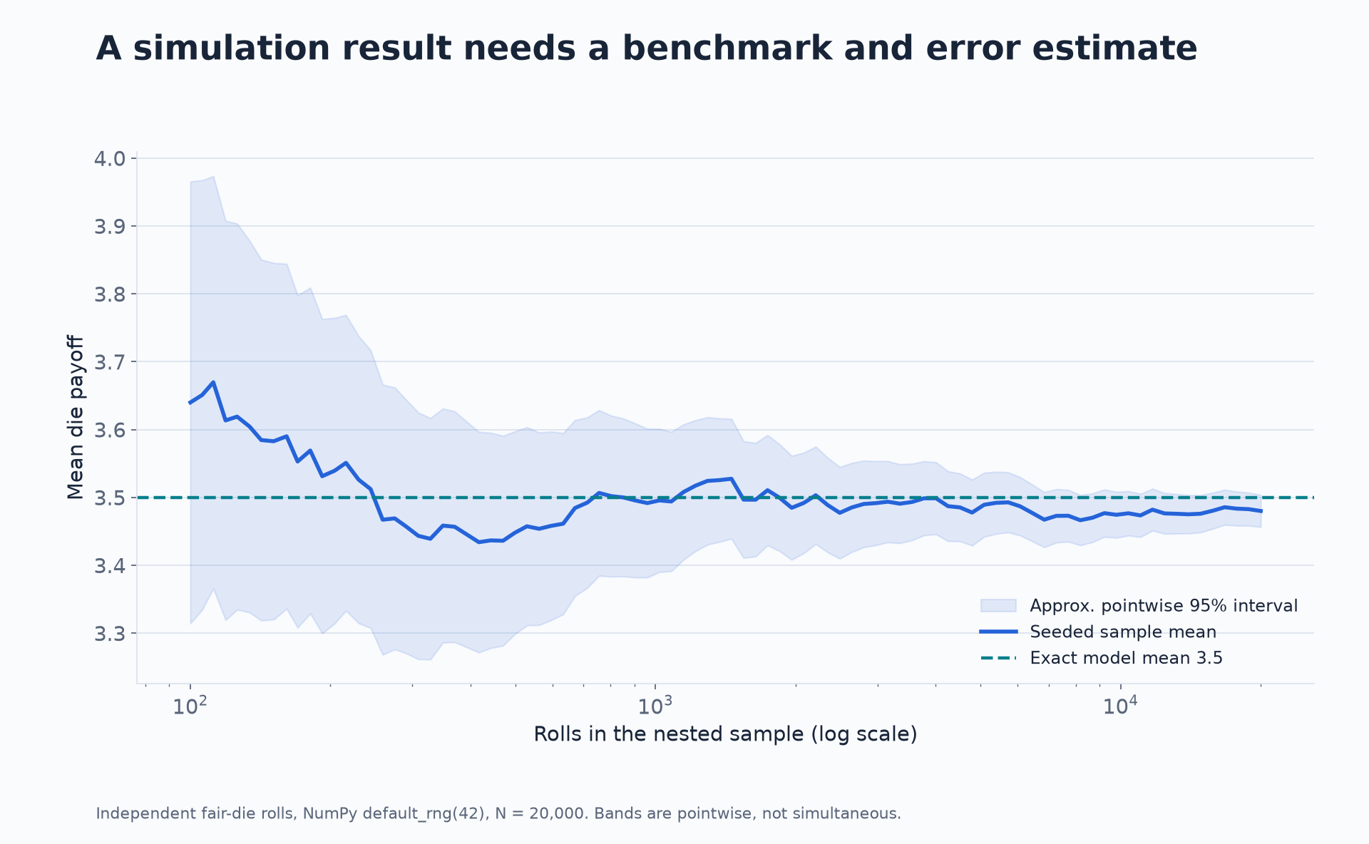
The exact variance of a fair die is $35/12$ , so the model standard error is $\sqrt{35/(12\times20,000)}\approx0.01208$ . The estimated value is consistent with that scale. The interval is a large-sample normal approximation, not a guarantee about every simulated run.

A seeded simulated die mean is compared with the exact mean and pointwise uncertainty bands as the nested sample grows.

Synthetic independent fair-die rolls, NumPy default_rng seed 42. Nested samples share observations; bands are pointwise, not simultaneous coverage.

Common mistake. Reinitialising the generator with the same seed inside every trial, which can repeat the same draw rather than create the intended independent sample. Another is interpreting extra sample size as a cure for an incorrectly specified distribution.

Follow-up. What does quadrupling the roll count do? It halves the theoretical standard error under independence. The realised absolute error need not decline monotonically.

Study simulation and resampling, statistical computation, and NumPy's generator documentation.

Question 5: debug a portfolio-risk calculation

Question. A 50/50 portfolio uses annual covariance matrix

\begin{pmatrix}0.04&0.01\\0.01&0.09\end{pmatrix}

. A function ignores the off-diagonal terms. What quantity does it miss, and what is the correct model volatility?

Hint. Expand

w^\top\Sigma w

, including both cross terms.

Solution. Correct variance is

0.25(0.04)+0.25(0.09)+2(0.5)(0.5)(0.01)=0.0375

. Volatility is its square root, approximately 19.3649% per year. Ignoring covariance gives variance 0.0325 and volatility approximately 18.0278%.

import numpy as np

weights = np.array([0.5, 0.5])
covariance = np.array([[0.04, 0.01], [0.01, 0.09]])
variance = float(weights @ covariance @ weights)
diagonal_only = float(np.sum(weights**2 * np.diag(covariance)))

print(f"Correct volatility: {100*np.sqrt(variance):.4f}%")
# Correct volatility: 19.3649%
print(f"Ignoring covariance: {100*np.sqrt(diagonal_only):.4f}%")
# Ignoring covariance: 18.0278%

Common mistake. Treating matrix multiplication that runs without an error as proof that dimensions and meaning are correct. For a reusable function, validate dimensions, finite entries, symmetry and the covariance matrix's numerical suitability. State the time unit of covariance and how weights represent positions.

Follow-up. Give an independent check. Set the portfolio to one asset: variance must equal that asset's diagonal covariance entry. Also compare a small hand-expanded two-asset formula with the matrix expression. These checks test meaning rather than duplicating the same matrix operation.

Read vectors, matrices and linear systems, eigenvalues and covariance matrices, and testing numerical code.

How to present a coding solution

Clarify the input contract, show a small baseline, then discuss complexity and necessary edge cases. If asked to optimise, identify what is expensive before changing the implementation. Keep time complexity, working storage and output storage distinct.

For data problems, define information timing and missing-value policies. For numerical problems, use units, benchmarks and limiting cases. For simulation, identify the distribution, generator, sample structure and uncertainty measure.

These examples practise a subset of interview work. Depending on the role, add algorithms, data structures, systems or domain-specific numerical problems. Jane Street's technology interview guidance provides one employer's preparation context; it does not establish a universal Python-only syllabus.

Continue with independent practice

Use programming and algorithms interview practice, Python for Quantitative Finance, and the preparation plan. Reattempt each problem on a changed fixture before moving on. If the solution only works for the printed numbers, inspect which assumption was hidden in the code.

For a larger simulation exercise with benchmark prices and variance reduction, continue to Monte Carlo option pricing with Python. The general Monte Carlo guide explains what its error bar measures.

Download the accompanying Python examples

Get the series code package. The download contains eight runnable Python solutions, an editable notebook and generators for eleven numerical charts. Use it to check a calculation after attempting the question, then practise a changed input or observation rule without consulting the solution. Downloads use the app’s usual email or member access.