Expected value interview questions: indicators, waiting times and stopping

Published 13 October 2026Updated 15 October 20267 min readQuant interview practice:Part 1 Part 2Part 3Part 4 Part 5 Part 6 Part 7

Expected value interview questions often become simpler when you choose the right representation. Use a probability-weighted sum for a small payoff, indicators for a random count, and a recurrence for a process whose next state determines what happens later. Linearity of expectation does not require independence; variance calculations and stopping arguments need their own assumptions.

We will solve five problems, from a single die payoff to consecutive patterns and a bounded stopping rule. The aim is to explain why a method works, then handle a follow-up that changes the model. These are teaching examples, not claims about a named employer's question bank.

If you are unsure what an observation means, begin with conditional probability interview questions. The interview overview connects this topic to the wider preparation sequence.

Question 1: value a small random payoff

Question. A fair six-sided die determines a game's net payoff: +8 if it shows six and −1 otherwise. Before any additional entry fee, what is the expected payoff? What is the largest extra fee a risk-neutral player could pay without making expected profit negative?

Hint. Use the stated net payoffs. Do not subtract the losing payment a second time.

Solution. There is one winning outcome and five losing outcomes:

\mathbb{E}[X]=\frac16\cdot8+\frac56\cdot(-1)=\frac12.

An additional deterministic fee $f$ changes expected profit to $0.5-f$ . The largest fee for nonnegative expected profit is therefore 0.5, under risk neutrality and ignoring other costs or constraints.

Common mistake. Treating a positive expectation as a sure gain. A single play loses one unit with probability

5/6

. Expected value describes the probability-weighted average, not the outcome of every play.

Follow-up. The variance is

\mathbb{E}[X^2]-\mathbb{E}[X]^2=(64+5)/6-0.25=11.25

. A constant entry fee changes the mean but leaves this variance unchanged. A risk-averse player need not be willing to pay the full expected value.

Study expectation, mean and variance. Financial valuation can require additional discounting and pricing assumptions; a physical expected payoff is not automatically a market price.

Question 2: count matches without listing every permutation

Question. Shuffle four labelled cards uniformly into four labelled slots. How many cards do you expect to land in their own slot? Generalise to

n

cards.

Hint. Count one card at a time, then add the counts.

Solution. Let

I_i

equal 1 if card

i

lands in its own slot and 0 otherwise. The number of matches is

X=\sum_i I_i

. Each card matches with probability

1/n

, so:

\mathbb{E}[X]=\sum_{i=1}^{n}\mathbb{E}[I_i]=n\cdot\frac1n=1.

The answer is one for every positive $n$ . The indicators need not be independent for linearity to apply.

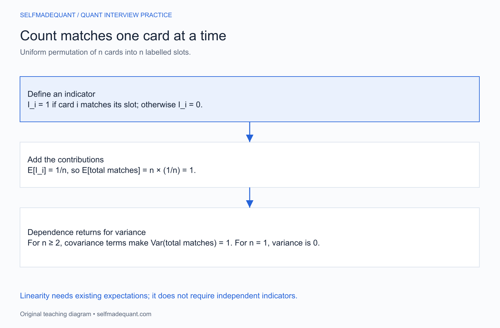
A random count is decomposed into card-match indicators; each contributes one over n to the expected total.

A uniform random permutation is the model. Dependence does not prevent adding expectations.

Common mistake. Assuming the expected value must be an outcome that occurs every time, or that indicators must be independent before they can be added. A permutation can have zero matches even though the expected count is one.

Follow-up. What is the variance? For

n\ge2

, two distinct cards both match with probability

1/[n(n-1)]

. The covariance terms matter:

\begin{aligned} \operatorname{Var}(X) &=\sum_i\operatorname{Var}(I_i)+2\sum_{i<j}\operatorname{Cov}(I_i,I_j)\\ &=\left(1-\frac1n\right)+\frac1n=1. \end{aligned}

For $n=1$ , the count is constant and variance is zero. Keep that boundary case separate.

For four cards, exact enumeration checks the mean and variance. Nine of the 24 permutations have no matches.

from itertools import permutations
from fractions import Fraction

counts = [sum(card == slot for slot, card in enumerate(order))
          for order in permutations(range(4))]
mean = Fraction(sum(counts), len(counts))
variance = sum((Fraction(x) - mean)**2 for x in counts) / len(counts)

print(mean, variance)
# 1 1
print(Fraction(counts.count(0), len(counts)))
# 3/8

Use expectation, variance and covariance to distinguish an expected total from its risk.

Question 3: how many destinations receive an order?

Question. Ten hypothetical orders independently choose one of five destinations, each with equal probability. What is the expected number of destinations receiving at least one order?

Hint. For each destination, find the probability it receives no orders.

Solution. A specified destination is missed by one order with probability

4/5

. Independence of the ten choices makes the probability it is empty

(4/5)^{10}

. Its occupancy indicator therefore has expectation

1-(4/5)^{10}

Adding across the five destinations gives:

\mathbb{E}[\text{occupied}]=5\left(1-\left(\frac45\right)^{10}\right)\approx4.4631.

Common mistake. Saying that the occupancy indicators are independent. They are not: knowing which destinations receive orders changes what can be true about the others. We used independent order choices to calculate an empty-destination probability, and linearity to add occupancy expectations. Those are different steps.

Follow-up. If destination

j

has routing probability

p_j

, with independent identical choices across orders, the expected occupied count is

\sum_j[1-(1-p_j)^{10}]

. Equal destination probabilities are no longer required. Real routing behaviour can violate the model's independence and fixed-probability assumptions.

A quick boundary check helps: zero orders occupy zero destinations; many orders with all $p_j>0$ push the expected count towards the number of destinations.

Question 4: why HH and HT have different waits

Question. Flip a fair independent coin repeatedly. Count flips through the first occurrence of HH. What is the expected count? How does it compare with waiting for HT?

Hint. Remember whether the latest flip leaves a partial match. Counting nonoverlapping pairs changes the experiment.

Solution for HH. Define state 0 as no trailing head and state H as one trailing head. Let

e_0

and

e_H

be the expected additional flips before completion. A step always costs one flip.

From 0, a tail returns to 0 and a head enters H. From H, a head finishes; a tail returns to 0. Thus:

\begin{aligned} e_0&=1+\tfrac12e_0+\tfrac12e_H,\\ e_H&=1+\tfrac12e_0. \end{aligned}

Substitution gives $e_0=6$ and $e_H=4$ . Starting fresh, HH takes six flips on average.

Solution for HT. State 0 behaves as before. From H, a tail now finishes and another head preserves H. Therefore

e_H=1+e_H/2=2

, and the state-0 equation yields

e_0=4

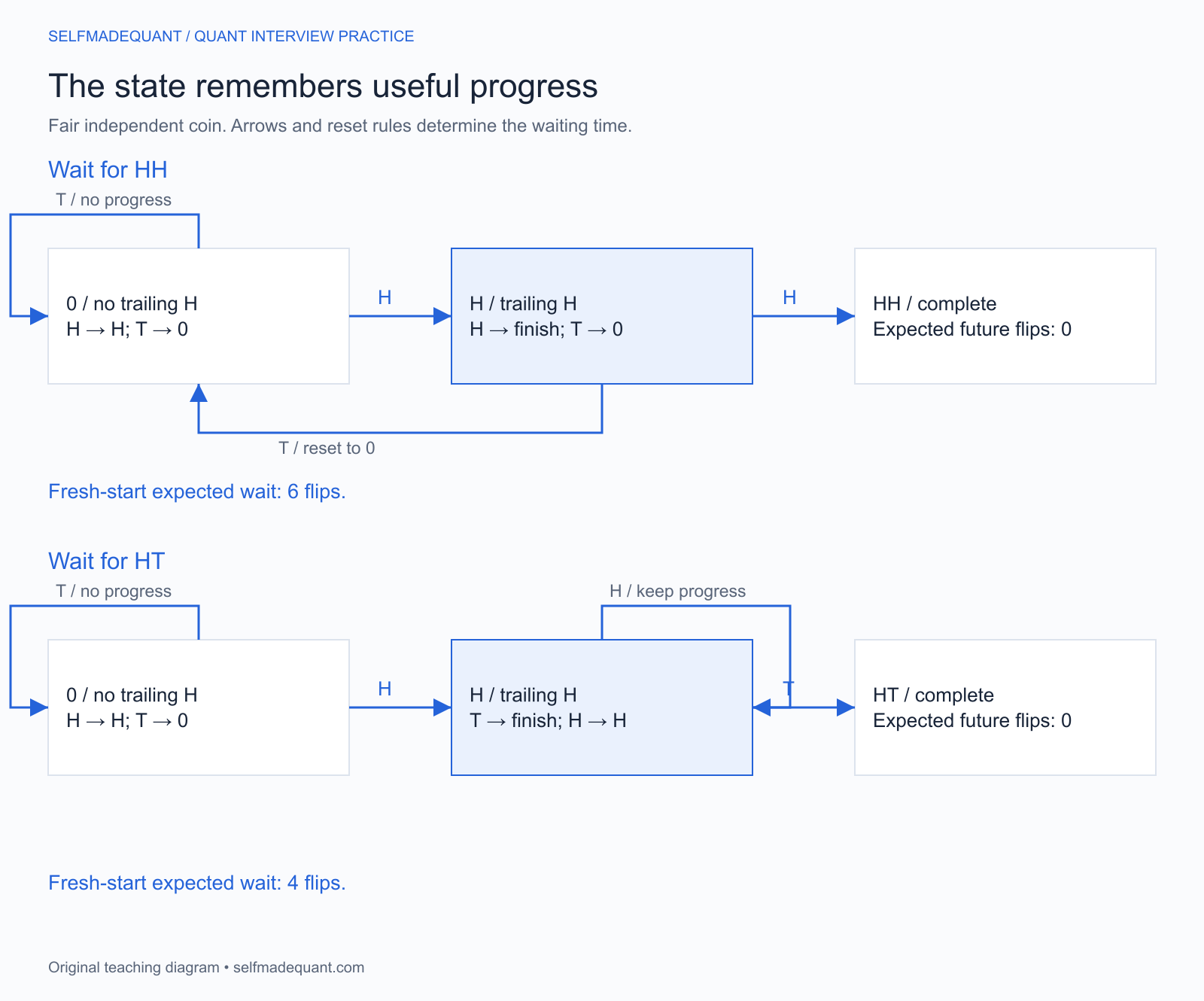
HH and HT use the same partial-match states but different transitions after a head; the resulting expected waits are six and four fair flips.

The state records usable progress. An H after H preserves progress for HT, while a T after H erases progress for HH.

Common mistake. Concluding that both waits equal four because either pattern has probability

1/4

in a prespecified pair. Successive candidate windows overlap. Pattern probability in a fixed window does not determine the first-occurrence waiting time by itself.

Follow-up. For independent flips with head probability

0<p<1

, the same recurrences give:

\mathbb{E}[T_{HH}]=\frac{1+p}{p^2},\qquad \mathbb{E}[T_{HT}]=\frac{1}{p(1-p)}.

At $p=1$ , HH arrives in exactly two flips, while HT never arrives. At $p=0$ , neither pattern arrives. These endpoints explain the domain restrictions rather than being numbers to substitute blindly into a formula.

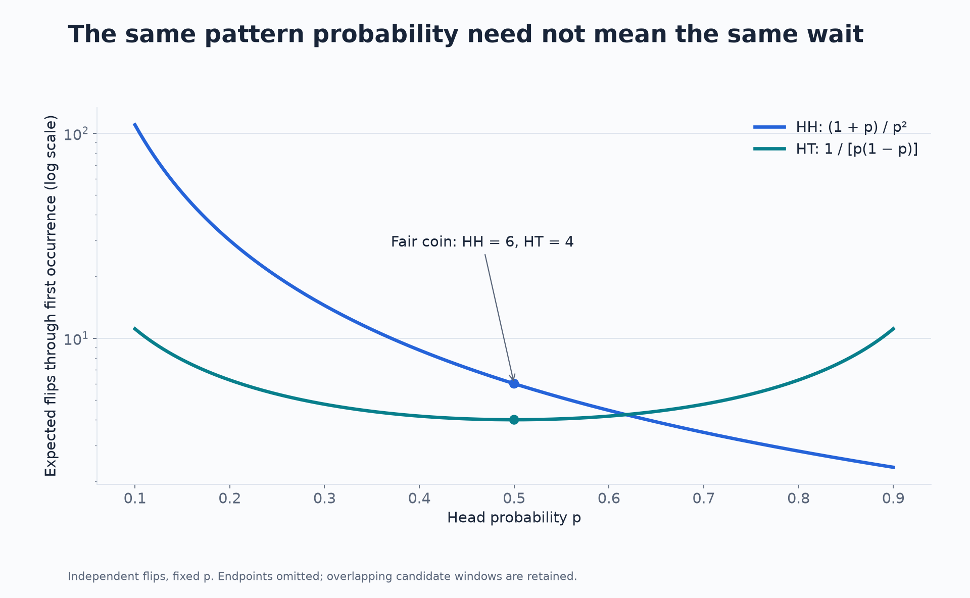
Analytic expected waiting times for HH and HT change differently as the independent coin's head probability changes.

Specified independent-coin model. The plot excludes endpoints where an expected wait can be infinite.

For a single head, the recurrence $e=1+(1-p)e$ gives $e=1/p$ . Check that you are counting trials through success; a convention counting only preceding failures gives $(1-p)/p$ .

Study conditional expectation and practise defining states before using a remembered waiting-time formula.

Question 5: does stopping after a win create profit?

Question. Independent fair coin flips pay +1 for heads and −1 for tails. Stop when cumulative profit first reaches +1, or after ten flips if that has not happened. What is expected terminal profit?

Hint. The choice to take the next flip depends only on the past, and there are at most ten flips.

Solution. Write terminal profit as the sum of up to ten possible payments, including payment

t

only if the game is still running just before flip

t

. Whether to include that payment is determined by earlier flips. Its next signed payoff still has conditional expectation zero.

Each included-payment term therefore has expectation zero, and a finite sum of them has expectation zero. The stopping rule changes the payoff distribution but not its expectation here.

Exact enumeration over all $2^{10}=1,024$ equally likely length-ten paths confirms the result. Later flips on a path that has already stopped are ignored.

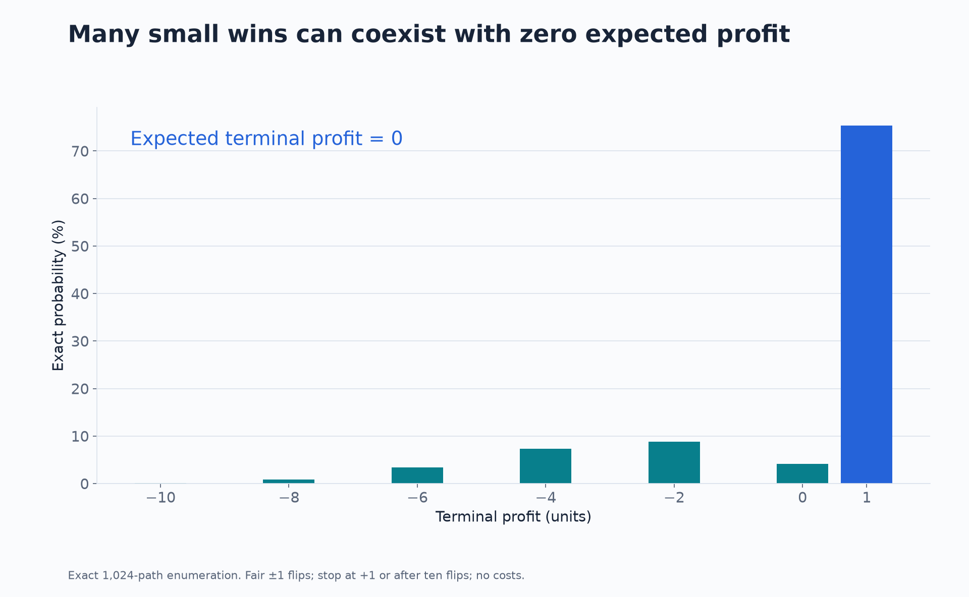
The bounded stopping rule produces many one-unit gains and less frequent larger losses; the exact expected terminal profit is zero.

Exact enumeration, fair independent flips, target +1 and ten-flip cap, no fees. Winning frequency alone does not determine expected profit.

The gain occurs with probability $193/256\approx75.39\%$ . Conditional on not reaching +1 by the cap, average terminal profit is $-193/63\approx-3.0635$ . The more frequent small wins are offset by the losing outcomes in expectation.

Common mistake. Pointing to the high winning frequency and ignoring loss sizes. Another mistake is removing the cap without re-examining the argument.

Follow-up. If you stop only upon reaching +1, the symmetric random walk reaches the target almost surely, but the expected time to do so is infinite. The bounded-sum argument no longer applies. Optional-stopping conclusions require their hypotheses; an almost-sure terminal gain is not by itself a valid argument that an implementable fair game has become profitable.

For an interview answer, the finite-cap proof above is enough to explain the stated problem. If you invoke a general martingale theorem, say which conditions justify it. MIT's optional-stopping teaching resource provides an external reference for that deeper distinction.

Check the method independently

Use exact enumeration when the sample space is small. For a waiting-time simulation, seed the generator, preserve partial matches between flips and report Monte Carlo standard errors across independent trials. A simulation supports an implementation check; it does not replace the recurrence's derivation.

The simulation and resampling lesson develops those checks. Harvard Stat 110 provides additional probability study, and Jane Street's probability playing-card page distinguishes introductory interview preparation from its much harder recreational problems.

Choose the representation before the formula

For a payoff, list outcomes and their probabilities. For a count, try indicators. For a repeated process, find the smallest state that determines the future law. For a stopping rule, identify what is known before each decision and whether the horizon is bounded.

Then change an assumption. Dependence, a different reporting mechanism or another stopping boundary can require a new calculation even when the story sounds similar.

Continue with Probability, Statistics and Financial Data and probability interview practice. The statistics problem set takes the next step: what can a finite sample tell you about an expectation?

To study the continuous-time connection behind fair-game reasoning, read martingales explained. It separates the conditional expectation property from the name of a betting system.

Download the accompanying Python examples

Get the series code package. The download contains eight runnable Python solutions, an editable notebook and generators for eleven numerical charts. Use it to check a calculation after attempting the question, then practise a changed input or observation rule without consulting the solution. Downloads use the app’s usual email or member access.