Statistics interview questions for quant researchers: five worked investigations

Published 15 October 20267 min readQuant interview practice:Part 1 Part 2 Part 3Part 4Part 5 Part 6 Part 7

Statistics interview questions for quant researchers test whether you can connect an estimate to its uncertainty, assumptions and evaluation design. A useful answer explains the sampling unit, the null or comparison, the role of dependence, and what the result can support. A small p-value or attractive backtest does not answer all those questions by itself.

We will examine confidence intervals, paired comparisons, multiple testing, serial dependence and information leakage. The numbers are illustrative, not observed investment results. Try each problem before reading its solution.

For probability foundations, use conditional probability and expected value. The interview overview shows where these statistical questions fit.

Question 1: an estimated mean and its uncertainty

Question. You have 100 independent observations with sample mean 0.001 and sample standard deviation 0.02, both in simple-return units. Calculate a large-sample approximate 95% confidence interval for the population mean. Does the estimate establish a positive mean?

Hint. Distinguish the dispersion of individual observations from uncertainty in their average.

Solution. The estimated standard error is:

\widehat{\operatorname{SE}}(\bar X)=\frac{0.02}{\sqrt{100}}=0.002.

Using the normal critical value 1.96, the interval is:

0.001\pm1.96(0.002)=[-0.00292,\;0.00492].

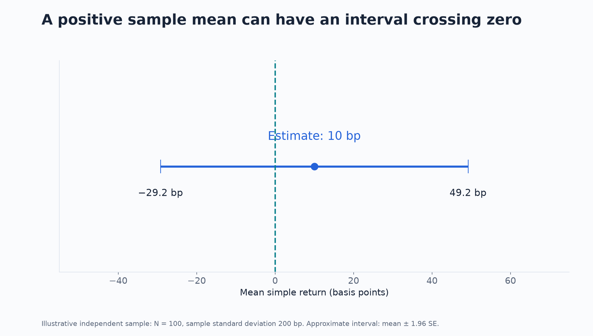
In basis points, the estimate is 10 bp, its standard error is 20 bp, and the interval is approximately [−29.2, 49.2] bp. It includes zero and negative means. The sample mean is positive, but this interval does not establish a positive population mean at the corresponding two-sided level under the approximation.

An estimated mean of ten basis points has an approximate confidence interval from minus 29.2 to 49.2 basis points under the independent-sample example.

Illustrative independent sample, N = 100 and sample standard deviation 200 bp. Normal approximation; no observed trading result.

Common mistake. Using 0.02 itself as the standard error, or saying there is a 95% frequentist probability that the fixed mean lies in this particular realised interval. The coverage statement concerns the interval procedure over repeated samples under its assumptions.

Follow-up. What changes for independent normally distributed observations with unknown variance? A Student t interval uses 99 degrees of freedom, giving a slightly larger critical value. For small, heavy-tailed or dependent financial samples, inspect the assumptions rather than automatically replacing one critical value with another.

Study confidence intervals and hypothesis testing. NIST's sample-size discussion explains how precision calculations depend on assumptions about variability and the desired error.

Question 2: compare forecasts on the same observations

Question. Two forecasting methods are evaluated on the same five independent cases. Define each loss difference as baseline loss minus candidate loss, so a positive number favours the candidate. The differences are

[2,1,-1,2,1]

. Compute the mean difference and a 95% t interval under an independent normal-difference model.

Hint. The observations for the comparison are the paired differences, not two unrelated samples of model losses.

Solution. Their sample mean is 1. The deviations from that mean are

[1,0,-2,1,0]

, whose squared sum is 6. With four degrees of freedom, sample variance is

6/4=1.5

, giving:

\operatorname{SE}(\bar d)=\sqrt{\frac{1.5}{5}}\approx0.5477.

The two-sided 95% t critical value with four degrees of freedom is approximately 2.7764. The interval is:

1\pm2.7764(0.5477)\approx[-0.5207,\;2.5207].

The sample favours the candidate on average, but this small-sample interval includes no improvement and negative improvement. The units are the units of the specified loss difference; they are not automatically return units or money.

from math import sqrt
from statistics import mean, stdev
from scipy.stats import t

differences = [2.0, 1.0, -1.0, 2.0, 1.0]
estimate = mean(differences)
standard_error = stdev(differences) / sqrt(len(differences))
critical = t.ppf(0.975, df=len(differences) - 1)

print(f"Mean difference: {estimate:.4f}")
# Mean difference: 1.0000
print(f"95% interval: [{estimate - critical*standard_error:.4f}, "
      f"{estimate + critical*standard_error:.4f}]")
# 95% interval: [-0.5207, 2.5207]

Common mistake. Ignoring the pairing and treating the methods as evaluated on unrelated cases. The variance of a difference includes the covariance between the two losses. Pairing can remove variation shared by both methods.

Follow-up. What if the five cases are consecutive dates with overlapping forecast outcomes? Independence is no longer automatic. The paired representation remains useful, but the simple standard-error and t-coverage arguments need reassessment.

See SciPy's paired-test documentation for the computational convention. For financial evaluation, study labels and overlapping outcomes and time-ordered validation.

Question 3: the best of one hundred tests

Question. You run 100 independent tests, all with true null hypotheses. Each test falsely rejects with probability 5%. What is the expected number of false rejections? What is the probability of at least one?

Hint. The expected count and the probability of a nonzero count are different quantities.

Solution. Write the false-rejection count as a sum of indicators. Its expectation is

100\times0.05=5

. Linearity does not require independence for that result, provided each marginal false-rejection probability is 5%.

For the probability of at least one false rejection, independence gives:

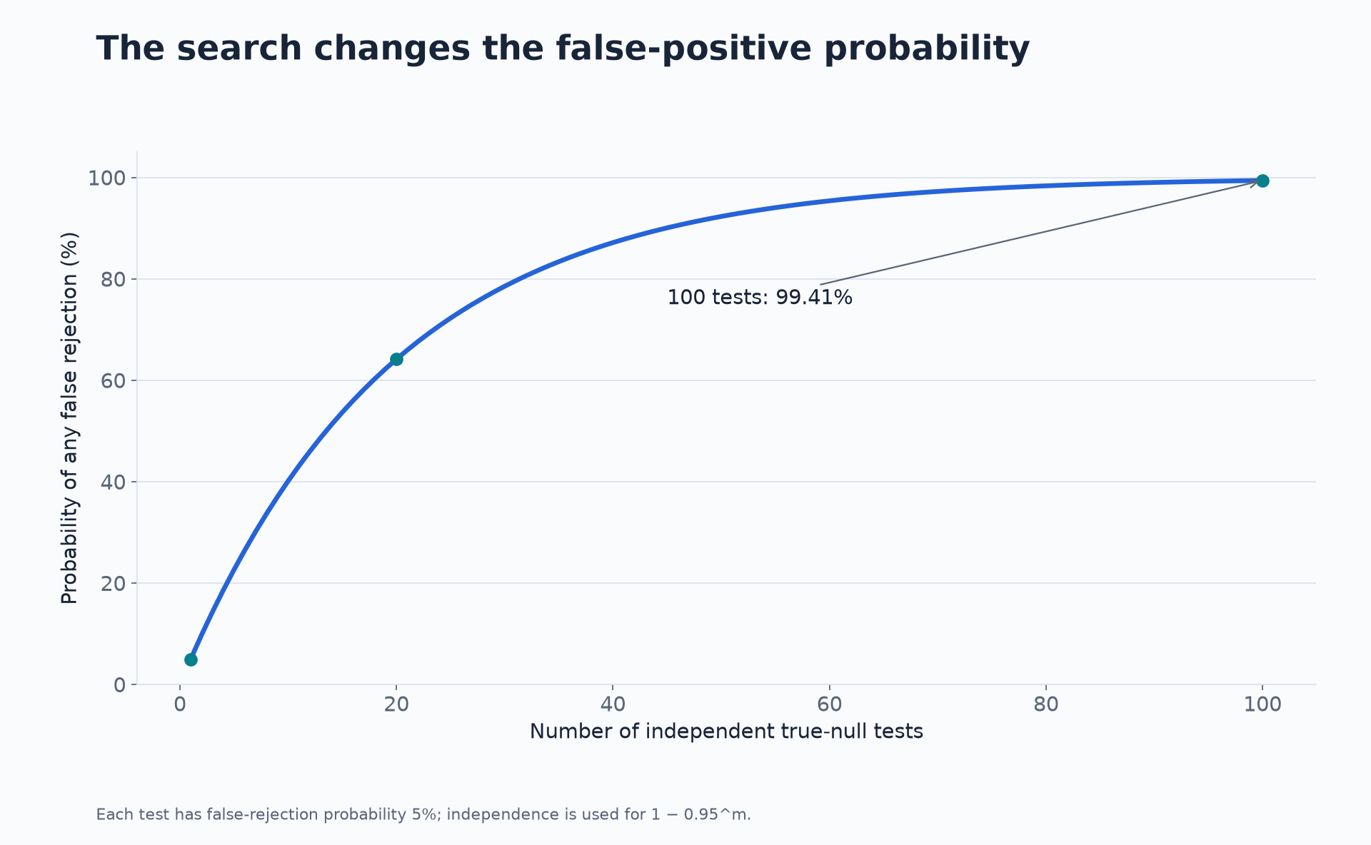
1-(1-0.05)^{100}=1-0.95^{100}\approx99.41\%.

Under independent true-null tests at five percent each, the probability of at least one false rejection rises with the number of tests.

Exact probability under the stated independent-test model. Correlated strategy variants need not follow this curve.

Common mistake. Interpreting an individual p-value of 0.03 as a 3% probability that the null is true. A p-value is a probability of results at least as extreme under the specified null and test, not a posterior probability of that null.

Another mistake is reporting only the winning strategy's test while hiding the search that produced it. The search includes feature choices, date ranges, universes and evaluation metrics, not only an explicit parameter grid.

Follow-up. Use a Bonferroni per-test threshold of

0.05/100=0.0005

. If the individual p-values are valid under their nulls, the union bound controls the probability of any false rejection at no more than 5%, without requiring independence.

This adjustment can be conservative. It does not repair leakage, an invalid test statistic or an unknown adaptive search history. NIST's Bonferroni discussion gives the probability inequality behind simultaneous control.

Use multiple testing and researcher degrees of freedom to connect the calculation to a research trial register.

Question 4: dependent observations and standard errors

Question. A stationary model has marginal variance

\sigma^2

and lag-

k

autocorrelation

\rho^k

, with

\rho=0.6

. For the average of 100 consecutive observations, how does its standard error compare with the independent-observation expression

\sigma/\sqrt{100}

Hint. Variance of a sum contains every pairwise covariance. Count how many pairs have each lag.

Solution. At lag

k

, there are

N-k

observation pairs. Therefore:

\operatorname{Var}(\bar X) =\frac{\sigma^2}{N}\left[1+2\sum_{k=1}^{N-1}\left(1-\frac{k}{N}\right)\rho^k\right].

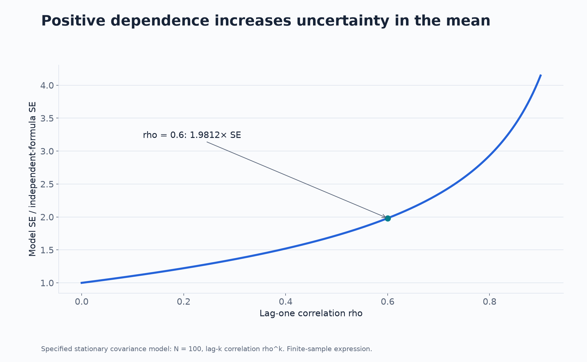
For $N=100$ and $\rho=0.6$ , the ratio of the correct model standard error to the independent expression is approximately 1.9812. An independent-formula standard error of 20 bp would become approximately 39.62 bp under this specified covariance model.

For large $N$ , the bracket approaches $(1+\rho)/(1-\rho)=4$ , giving an approximate factor of two in standard error. The finite-sample expression gives the more precise value here.

The finite-sample standard-error inflation factor for a mean increases with positive autocorrelation in a specified stationary covariance model.

N = 100, autocorrelation at lag k equal to rho to the power k. A teaching model, not an estimate of a particular return series.

Common mistake. Treating 100 dates as 100 independent pieces of information. Another is confusing the variance multiplier, about four, with the standard-error multiplier, about two.

Follow-up. What if you do not know the dependence structure? Estimate uncertainty using a method appropriate to the experiment, such as a justified dependence-robust variance estimate or block resampling. State its assumptions and assess sensitivity. Plugging an estimated autocorrelation into this formula does not make the model exact.

Study joint distributions and dependence, financial return characteristics and simulation and resampling.

Question 5: a strong model with impossible information

Question. A daily trading model uses a company's final reported quarterly value on every date in that quarter. A random train/test split gives excellent accuracy. What should you investigate before discussing the score?

Hint. Ask when the value became available and what the validation split permits the model to learn.

Solution. The quarter label is not the release timestamp. If the value was published later, using it inside the quarter leaks future information into historical decisions. Later revisions can introduce additional hindsight.

A random row split can also mix nearby dates, overlapping labels or repeated entities in ways inconsistent with the intended deployment. It may make evaluation easier than a future prediction problem.

Reconstruct observation, release, decision and feasible execution times. Use data versions available at each historical decision. Choose time-ordered training, validation and final evaluation that reflect the target task, with additional handling for overlap when required. Fit transformations and feature selection using only the permitted training information.

Common mistake. Trying another model or adding regularisation before repairing the information set. Statistical sophistication cannot make unavailable data available.

Follow-up. What if performance collapses after the repair? Report that result. Preserve the original run, explain the bug and distinguish the corrected experiment from a new search for favourable parameters. A failed original hypothesis can still yield a useful research conclusion.

Read observation, event and availability timestamps, point-in-time data, and purging and embargoes.

What a strong statistical explanation includes

Identify the sampling unit, quantity being estimated, comparison or null, independence assumptions, and evidence of model selection. Put the effect size and uncertainty before a yes/no significance label. Then connect the result to the financial decision and its costs.

You do not need to recite every possible diagnostic. Name the assumption most likely to change the interpretation, explain how it could fail and propose a specific check.

For external study, use Harvard Stat 110 for probability and StatQuest's video index for focused statistical explanations. Neither watching a video nor running a library test replaces checking that the procedure matches your experiment.

Continue from the gap you found

Use statistics interview practice, paired with Probability, Statistics and Financial Data. For research design, continue into Quantitative Research, Data and Backtesting. The preparation plan shows how to combine worked questions, concept repair and unfamiliar follow-ups.

Download the accompanying Python examples

Get the series code package. The download contains eight runnable Python solutions, an editable notebook and generators for eleven numerical charts. Use it to check a calculation after attempting the question, then practise a changed input or observation rule without consulting the solution. Downloads use the app’s usual email or member access.