Conditional probability interview questions ask you to update probabilities after receiving information. The decisive step is defining exactly what was observed and how it was reported. Count equally likely outcomes only when your model justifies equal weights; use Bayes' rule when the observation is more likely under some hidden states than others.
Two fair dice can produce an answer of 1/11 or 1/6 to superficially similar questions. The difference is the conditioning event, not a different formula. We will use that distinction to solve four connected problems, including a screening signal and a hidden-bag experiment.
These are teaching problems, not leaked or firm-attributed interview questions. Attempt the question before its hint and solution. For the wider practice map, read quant interview questions and answers.
Question 1: at least one die is a six
Question. Roll two fair independent six-sided dice. You are told, truthfully and using the rule “report whether at least one six is present,” that at least one die is a six. What is the probability both dice are six?
Hint. Label the dice first and second, then draw the ordered outcome grid.
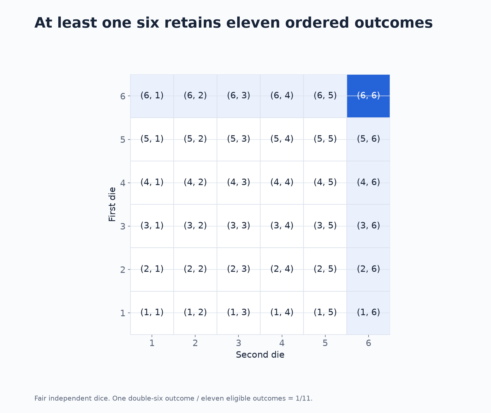
Solution. Before the observation there are 36 equally likely ordered pairs. The event “first die is six” contains six pairs; “second die is six” contains six. Their intersection, (6,6), was counted twice, so the union contains 6+6−1=11 pairs.
One of those eleven pairs has both dice equal to six. Therefore:
P(both six∣at least one six)=111.
An ordered two-dice grid highlights the eleven outcomes with at least one six and identifies the single double-six outcome.
Fairness and independence make the 36 original ordered outcomes equally likely. The stated reporting rule retains eleven of them.
Common mistake. Saying “the other die has probability 1/6” without identifying which die the report establishes as a six. The conditioning event did not select a particular die.
Another mistake is counting 21 unordered pairs as equally likely. An unordered pair such as {1, 6} represents two ordered outcomes; {6, 6} represents one. Unordered representations can work, but their weights must differ.
Follow-up. Suppose instead you are told that the first die is six. Six ordered pairs remain, and one is (6,6). The answer becomes 1/6.
Question. Roll the same two dice. Independently choose one die with a fair coin and inspect it. You hear that the inspected die shows six. What is the probability both dice show six?
Hint. Include the inspected index in the experiment. The report is not equally likely for every pair containing a six.
Solution. There are 72 equally likely triples: first die, second die and inspected index. Twelve produce a six report. Two of those correspond to (6,6), because inspecting either die produces the report.
The conditional probability is 2/12=1/6.
Equivalently, let A mean both dice are six and R mean the inspected die is six. Then P(R)=1/6, and P(A∩R)=1/36, because the report is certain when both dice are six. Their ratio is 1/6.
Common mistake. Reusing the eleven surviving pairs from question 1 and assigning them equal conditional weights. A pair with exactly one six produces the report only half the time, whereas (6,6) produces it every time. Conditioning changes their relative weights.
Follow-up. What if the reporter inspects both dice and reports “six” whenever either is six? That is question 1's event, giving 1/11. The observation mechanism belongs in the model.
Here is an exact enumeration. It has no simulation error and needs no random seed because it enumerates the entire finite experiment.
from itertools import product
from fractions import Fraction
reports = []
for first, second, inspected in product(range(1, 7), range(1, 7), (0, 1)):
dice = (first, second)
if dice[inspected] == 6:
reports.append(first == second == 6)
print(len(reports), sum(reports))
# 12 2print(Fraction(sum(reports), len(reports)))
# 1/6
The code checks the model you wrote. It cannot decide whether that model matches an ambiguously worded question. Clarifying the observation comes before enumeration.
Question 3: reverse a screening probability
Question. In a hypothetical population, 2% of events belong to a category of interest. A screen alerts on 90% of category events and 5% of all other events. Given an alert, what is the probability the event belongs to the category?
Hint. Work with expected counts in a representative population of 10,000 events.
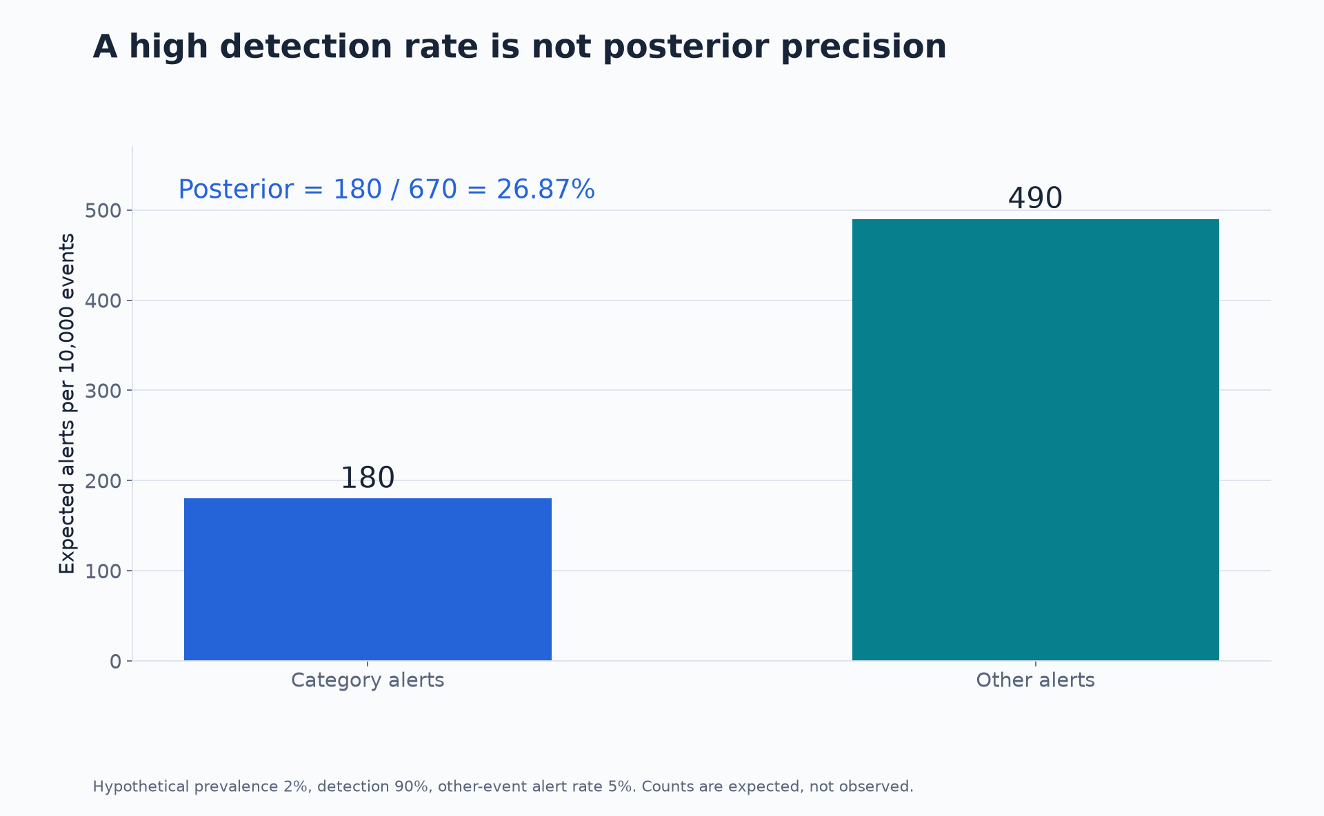
Solution. The population contains 200 category events and 9,800 others in expectation. The screen produces 180 category alerts and 490 other alerts. Out of 670 alerts, 180 belong to the category:
Expected counts from a hypothetical screen: 180 alerts from category events and 490 alerts from other events.
Hypothetical rates and expected counts, not measured signal performance. Realised finite-sample counts would fluctuate.
Common mistake. Reporting 90%. Detection probability P(alert∣category) is different from the requested posterior probability P(category∣alert).
Ignoring the large outside population also fails: its modest false-alert rate still generates more alerts than the category does.
Follow-up 1. If the false-alert rate falls to 1%, with prevalence and detection unchanged, the expected other alerts fall to 98. The posterior becomes 180/(180+98)=90/139≈64.75%.
Follow-up 2. If prevalence rises to 10% while the original 90% detection and 5% false-alert rates remain valid, the posterior becomes 0.09/(0.09+0.045)=2/3.
The screen has the same conditional rates in the second follow-up, yet precision changes. That is why a posterior calibrated in one population need not transfer to a population with another prevalence.
Use odds as a separate check
Prior odds are 0.02/0.98=1/49. The alert likelihood ratio is 0.90/0.05=18. Posterior odds are therefore 18/49, which convert to probability 18/(18+49)=18/67.
If your count calculation and odds calculation disagree, inspect which probability conditions on which event. The Bayesian reasoning lesson develops these updates.
In a financial application, this posterior is still not a profitability statement. You must define the category, forecast horizon, payoff, costs and information available at the decision. A signal selecting a group of events changes the group you analyse; it does not automatically make that group economically useful.
Question 4: a hidden bag and a second draw
Question. Choose one of two bags with equal probability. Bag A contains two red balls and one blue; bag B contains one red and two blue. Draw a ball uniformly and observe red. What is the probability you chose A? If you draw again without replacement from the same bag, what is the probability the second ball is red?
Hint. Update the bag probability, then use the composition remaining in each bag.
Solution, first part. Red is twice as likely under A as under B. The marginal probability of red is:
21⋅32+21⋅31=21.
Bayes' rule gives:
P(A∣red)=2121⋅32=32.
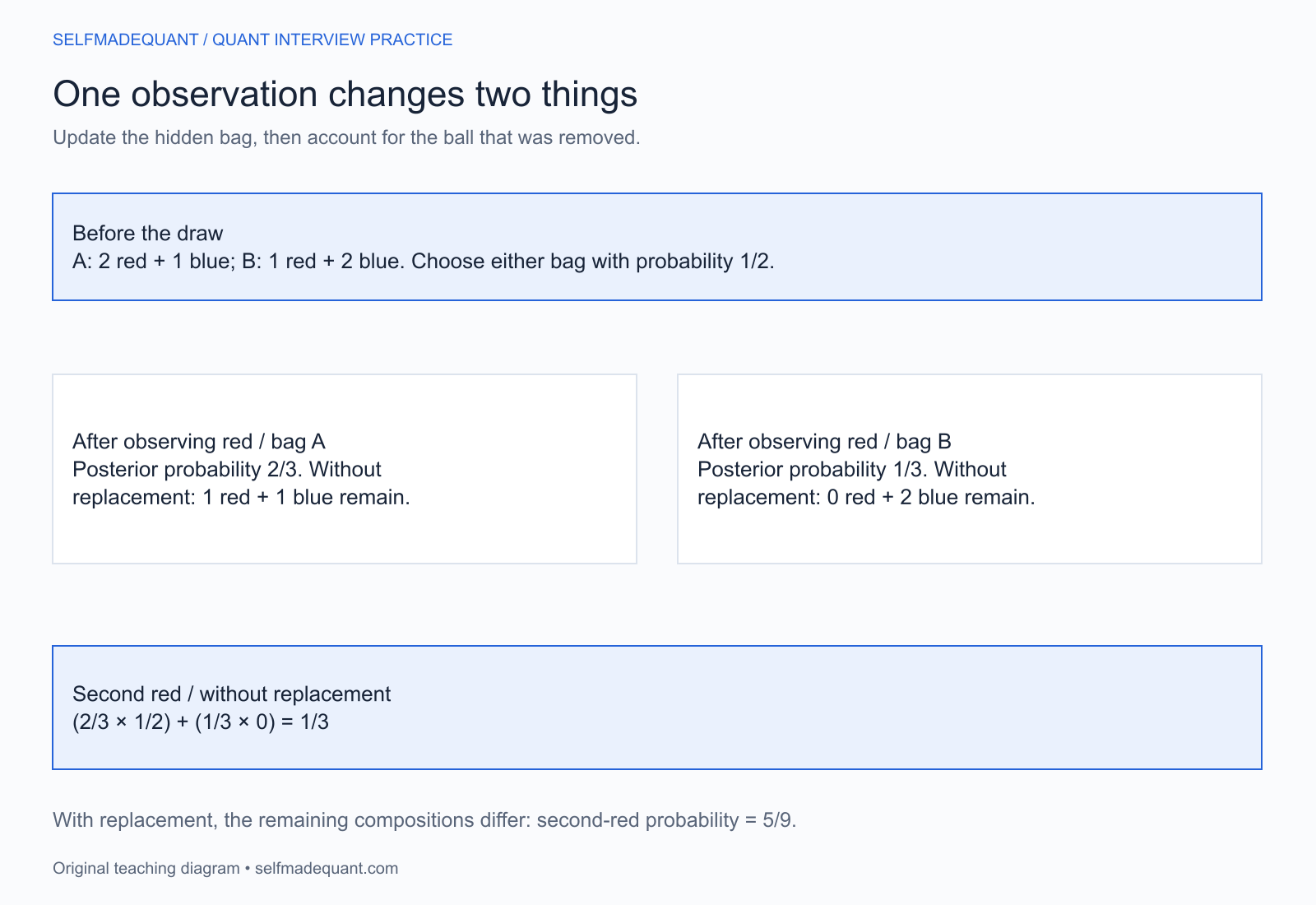
Solution, second part. If A was chosen, observing and removing a red ball leaves one red and one blue, so the next red probability is 1/2. If B was chosen, no red balls remain. Weight those probabilities by the updated bag probabilities:
P(second red∣first red)=32⋅21+31⋅0=31.
The first red draw updates the bag probabilities to two-thirds for A and one-third for B; without replacement, the next red probability is one-third.
Two updates are required: which bag is more likely, and which balls remain within each bag.
Common mistake. Updating the bag probability but using its original composition for a draw without replacement. That would calculate a different experiment.
Follow-up. Replace the first ball before drawing again. Conditional on a known bag, the two draws are now independent. But with the bag hidden, the first draw still teaches you which bag is more likely. The second red probability becomes:
32⋅32+31⋅31=95.
Conditional independence given a hidden state does not imply unconditional independence. Conversely, removing a ball introduces another dependence mechanism. State which experiment you are analysing.
Begin with the experiment, observation rule and requested event. Then say whether you are counting outcomes, weighting likelihoods or conditioning on a hidden state. Define the denominator before substituting numbers.
Give an independent check when it is cheap: enumerate a finite experiment, use expected counts, or update odds. If asked to simulate, seed the random generator and report simulation uncertainty. For a small finite sample space, exact enumeration is usually a stronger implementation check.
When the wording is ambiguous, offer the answer under each plausible observation mechanism. That is more useful than guessing which memorised puzzle the question resembles.
Practise a changed assumption
Revisit the questions with biased dice, unequal bag probabilities or another category prevalence. Write the new likelihoods before calculating. Then explain whether the original answer should rise or fall.
Do not multiply conditional likelihoods for repeated reports unless you can justify their conditional independence. Two alerts from systems using the same input data may contain much less additional information than two independent observations.
Get the series code package. The download contains eight runnable Python solutions, an editable notebook and generators for eleven numerical charts. Use it to check a calculation after attempting the question, then practise a changed input or observation rule without consulting the solution. Downloads use the app’s usual email or member access.
Go deeper with lessons, derivations and worked exercises behind this article.