Market-making interview questions ask you to connect a quote with the trades and risks it creates. Calculate from the market maker's perspective, condition on the information in a fill, track inventory, and distinguish a displayed spread from realised profit. A useful answer states the payoff model, customer behaviour, size and costs before choosing a price.
We will use a small random contract, then add informative flow, inventory and an order-book execution. These are original teaching scenarios, not a model of a particular firm's strategy or claims about its interview questions.
Jane Street's Probability & Markets page explains why probability, expectation and making markets appear in its preparation material. Its mock trading interview is a useful example of discussing a problem as assumptions change. Our calculations below stand on their stated models.
Question 1: make a two-sided quote
Question. A contract pays 40 or 60, each with probability one half. Ignore discounting, fees, financing and counterparty risk. You quote bid 49 and ask 51 for one contract. A customer buys from you, and their choice contains no information about the payoff. What is your expected profit and possible realised profit?
Hint. A customer's purchase is your sale. Track the cash received and settlement owed.
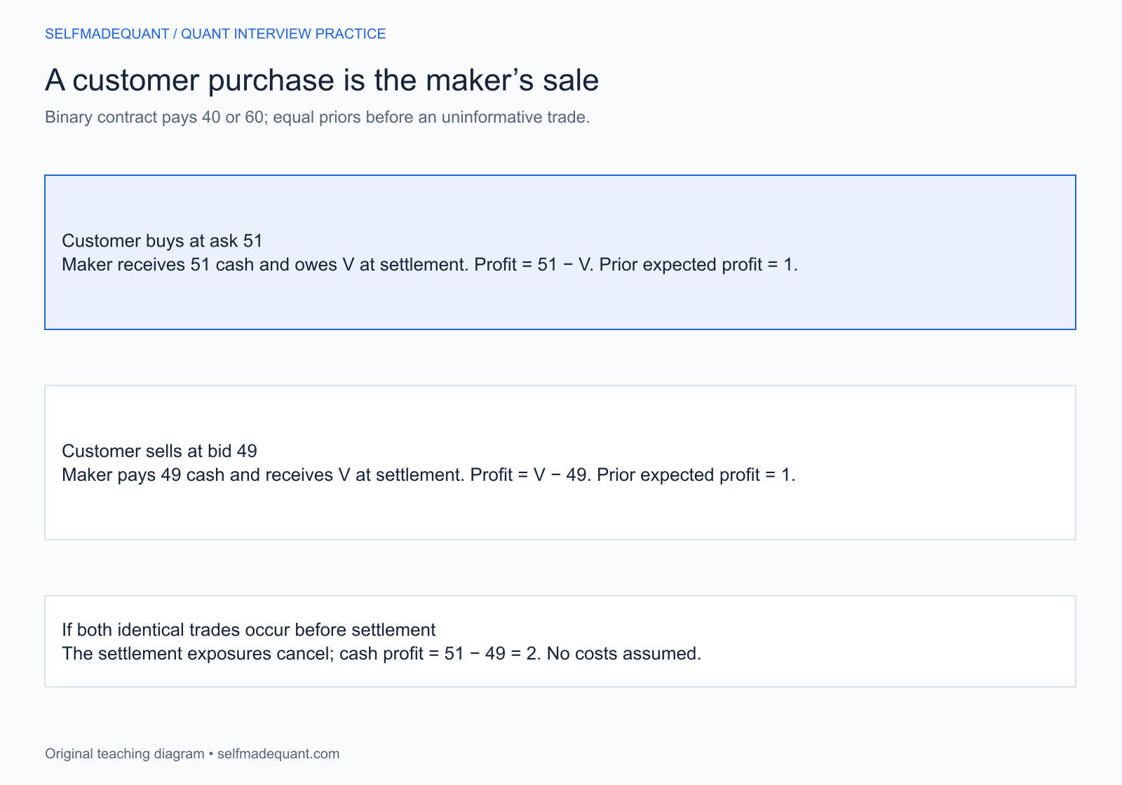
Solution. You receive 51 and owe the settlement value V. Your profit is 51−V. The expected payoff is 50, so expected profit is 1. If V=40, you gain 11; if V=60, you lose 9.
The bid–ask spread is 2, but that is not the profit on this one unhedged sale.
When a customer buys at the ask, the market maker receives cash and owes the eventual contract payoff; when a customer sells at the bid, the maker pays cash and owns the payoff.
Specified binary payoff, one contract, no fees or financing. Follow the transfers from the maker's perspective.
Common mistake. Saying “buy at 49 and sell at 51” as though both trades have already happened. The question gives only a sale. You may carry a short position while waiting for an offsetting trade.
Follow-up. Suppose you also buy an identical contract at 49 before settlement. The long and short payoffs cancel, leaving cash profit 2 under these assumptions. If the contracts differ in expiry or settlement, cancellation need not hold.
Question. Keep the contract's prior probabilities equal. Now a customer buys with probability 0.8 when V=60 and 0.2 when V=40. Evaluate your expected profit conditional on selling at the ask of 51. What zero-expected-profit ask would match this conditional payoff in the toy model?
Hint. Update the probability of the high payoff after observing a buy.
Solution. Bayes' rule gives:
P(V=60∣buy)=0.8⋅0.5+0.2⋅0.50.8⋅0.5=0.8.
Conditional expected settlement is 0.8(60)+0.2(40)=56. At an ask of 51, expected profit per received buy is 51−56=−5.
An ask of 56 would give zero expected profit on that conditional settlement distribution, before costs. If the complementary sell probabilities are 0.2 in the high state and 0.8 in the low state, the corresponding conditional value after a sell is 44.
These are conditional break-even values, not a solved trading equilibrium. The stated customer probabilities describe the toy flow; changing the quote can change actual customer behaviour, fill probability and competition. Do not assume the same probabilities remain economically valid at every new price.
Common mistake. Using the prior value of 50 after a trade that selects high-value outcomes. The inventory you receive is a selected sample, not a random draw independent of value.
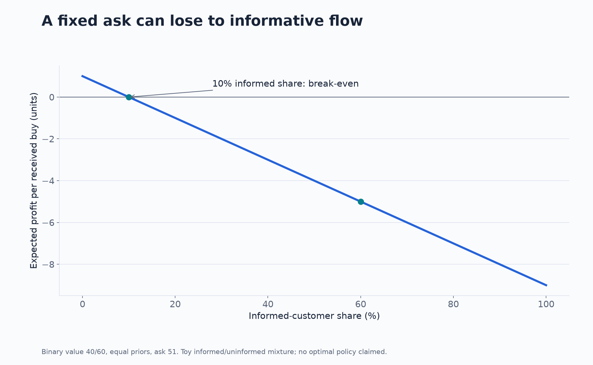
Follow-up. Suppose a fraction α of arriving customers are informed: they buy in the high state and sell in the low state. The rest independently buy or sell with equal probability. Under equal prior states, conditional high-state probability after a buy is (1+α)/2.
Conditional expected value becomes 50+10α, and at the fixed ask of 51, expected profit per buy is 1−10α. It reaches zero at α=0.1. With α=0.6, the original 0.8/0.2 buy probabilities return and expected profit is −5.
In a specified mixture of informed and uninformed customer flow, expected profit per buy at a fixed ask declines as the informed share rises.
Binary payoff 40/60, equal priors, fixed ask 51 and exogenous toy flow. The curve is not an estimated market relationship or an optimal quoting policy.
Question. You bought three contracts at 49. They all settle to the same binary value, 40 or 60. What is the terminal profit distribution? If you sell two identical contracts at 50 before settlement, how does it change?
Hint. These are three exposures to one settlement value, not three independent payoffs.
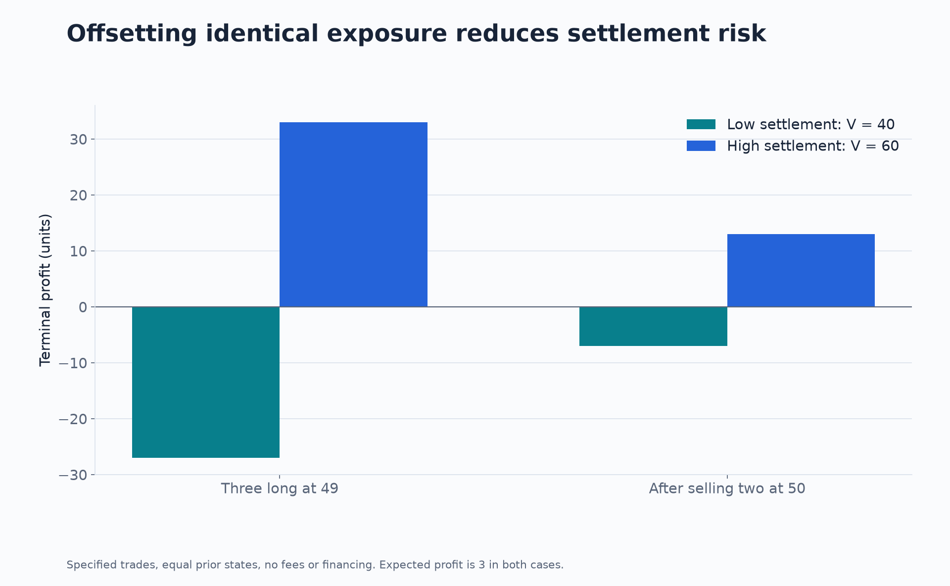
Solution before the sale. You paid 147 and own three contracts. Terminal profit is 3V−147, so the outcomes are −27 and +33. Expected profit is 3 under equal prior states.
Solution after the sale. Selling two contracts brings in 100, leaving net cash paid of 47 and one contract's settlement exposure. Profit is now V−47, giving −7 or +13. Expected profit remains 3 under this simplified no-cost transaction sequence, while the exposure to settlement uncertainty is smaller.
Selling two of three identical long contracts reduces the spread between low-state and high-state terminal profit outcomes while leaving the toy-model expectation unchanged.
Specified equal-prior payoff model and stated trade prices, no costs. The offsetting sale is assumed available; it is not guaranteed by the earlier quote.
Common mistake. Claiming that the three positions diversify because there are three contracts. Their settlement values are identical, so their gains and losses move together.
Follow-up. How might a long inventory affect a simple quote rule? As an illustrative skew, shift a reference midpoint from 50 to 50−0.5q, with inventory q and fixed half-spread 1. At q=3, the rule quotes 47.5/49.5. Its lower bid discourages additional buying by the maker, while its lower ask can encourage customer purchases that reduce the maker's inventory.
This rule is a demonstration of direction, not an optimal policy. It does not force customers to trade, account for informative flow, or replace risk limits. An inventory skew can also worsen one objective while improving another.
Question. A static book has best bid 99.95 and these asks: two units at 100.05, three at 100.10 and five at 100.30. You buy four units. What is your average execution price and cost relative to the initial midpoint of 100? Add a fee of 2 bp of executed notional.
Hint. The second price level is only partially consumed. Keep the fee base explicit.
Solution. Buy two units at 100.05 and two at 100.10. Executed notional is:
2(100.05)+2(100.10)=400.30.
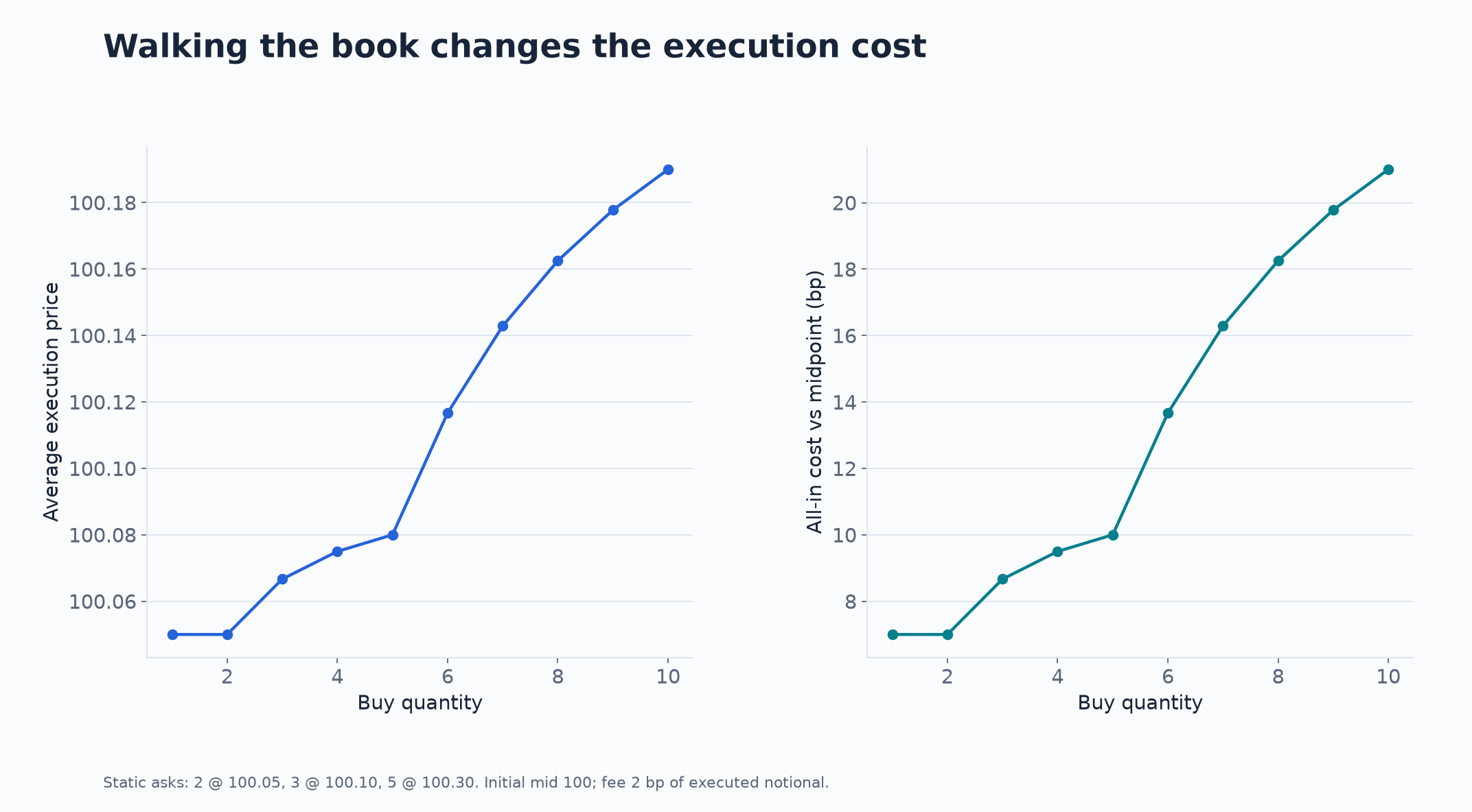
The volume-weighted average price is 400.30/4=100.075. Against reference notional 4×100=400, the price concession is 0.30, or 7.5 bp.
The fee is 400.30×0.0002=0.08006. Total cost relative to the midpoint is 0.38006, which is:
4000.38006×10,000=9.5015 bp.
Simply adding 7.5 and 2 gives the approximation 9.5 bp. The tiny difference arises because the fee is charged on executed notional rather than midpoint reference notional.
Average execution price and all-in cost rise as a hypothetical buy consumes successive levels of a fixed ask book.
Static displayed book, zero latency, no hidden liquidity or market reaction. Fees equal 2 bp of executed notional; cost is measured against initial midpoint notional.
Common mistake. Charging the full requested quantity at the best ask, or confusing the initial midpoint with an executable price. Also state whether a “cost” includes fees and which notional is its denominator.
Follow-up. What if the requested quantity is eleven? The displayed asks contain only ten units. A complete eleven-unit execution cannot be priced from this snapshot. Specify rejection, partial execution or an additional liquidity assumption; do not silently invent an eleventh unit at the last displayed price.
State whose buy or sale is being described, what settles, which positions remain and what information the trade contains. Separate a conditional profit per fill from expected profit per submitted quote: the latter also depends on fills and the nonfill branch.
If a market changes after the quote, reconstruct the event order rather than evaluating an earlier decision using knowledge that arrived later. If a static book is all you have, say what it cannot reveal about queue position, cancellations or your own impact.
Practise the next variation
Change one element at a time: the payoff probabilities, informed-flow share, inventory, quoted size, fee or available depth. Recompute cash and positions before discussing strategy. A new parameter can expose whether you understood the transfers or only remembered the answer.
Get the series code package. The download contains eight runnable Python solutions, an editable notebook and generators for eleven numerical charts. Use it to check a calculation after attempting the question, then practise a changed input or observation rule without consulting the solution. Downloads use the app’s usual email or member access.
Go deeper with lessons, derivations and worked exercises behind this article.