The maths of market making: value, information, inventory, and fills

Published 4 October 2026Updated 10 October 20267 min readMarket making:Part 1Part 2Part 3

Suppose you know how to quote a two-sided market. You can explain the bid and ask, calculate the profit on a trade, and explain why holding more inventory changes your next decision.

But how do you calculate a new value after information arrives? How much risk does an extra contract add? And what happens when a wider spread gives you a larger margin but fewer trades?

In Part 1, we explored those questions through a die contract. This time, we will put numbers to them and connect the calculations to the mathematics you can study on SelfMadeQuant.com.

Let’s start with the four-dice contract in my free Market Making game.

First, calculate what you know

The contract pays the sum of four fair, independent dice:

V=D_1+D_2+D_3+D_4.

Each die has mean $3.50. By linearity of expectation, the expected sum is:

\mathbb{E}[V]=4(3.50)=14.

Now the first die is publicly revealed as 6. The remaining three are still unknown:

\mathbb{E}[V\mid D_1=6]=6+3(3.50)=16.50.

Replace the first die’s expected payoff with its observed value. Keep the expected payoffs of the three independent, unseen dice unchanged.

This is conditional expectation: an average calculated using the information currently available.

The game also has a card version. The game deals cards without replacement. Seeing one card therefore changes which cards remain in the deck. If a high card is removed, the remaining average falls. That is a reason to study independence: the unseen dice keep their original distributions, while the remaining cards depend on what has already been drawn.

The trade itself changes what you should believe

In the one-die example, an uninformed customer's purchase did not change our expected payoff of $3.50. A perfectly informed customer's purchase at our $4 ask restricted the result to 5 or 6.

The relevant expected payoff became:

\mathbb{E}[V\mid\text{informed customer buys at }4]=5.50.

Evaluate a quote using the outcomes you expect when that quote fills. A fill means that your order has traded.

For a passive purchase at bid $b$ , the expected settlement profit is:

\mathbb{E}[V-b\mid\text{your bid fills}] =\mathbb{E}[V\mid\text{your bid fills}]-b.

Consider an invented stock example. The midpoint is $100, and you bid $99.99. Conditional on your bid filling, assume that the midpoint one second later is:

$99.96 with probability 70%.
$100.02 with probability 30%.

The conditional expected future midpoint is:

0.7(99.96)+0.3(100.02)=99.978.

Your expected marked profit is therefore:

99.978-99.99=-0.012

per share, before costs. You bought one cent below the old midpoint. The expected later price move more than removes that initial advantage.

The probabilities are assumptions for this example. To estimate them, collect data on comparable fills and later prices. Bayes’ rule expresses how evidence changes probabilities. You still need inputs for those probabilities.

The same logic explains a partially informed trader in the four-dice game. After the first die is revealed as 6, the public estimate is $16.50. Suppose an insider also knows that the fourth die is 1. Their estimate is:

6+1+2(3.50)=14.

If you bid $15.50, they can sell to you at a price above their conditional estimate. They do not need to know the final sum to have an information advantage.

How much uncertainty remains?

An expected value tells us an average. Variance and standard deviation describe variation around that average.

For one fair die:

\begin{aligned} \mathbb{E}[D^2]&=\frac{1^2+2^2+3^2+4^2+5^2+6^2}{6}=\frac{91}{6},\\ \text{Var}(D)&=\mathbb{E}[D^2]-\mathbb{E}[D]^2=\frac{35}{12},\\ \text{SD}(D)&=\sqrt{\frac{35}{12}}\approx1.708. \end{aligned}

Because the four dice are independent, their variances add. After each public reveal, one fewer random die remains:

Publicly revealed dice	Unknown dice	Conditional variance of the sum	Conditional standard deviation
0	4	11.667	3.416
1	3	8.750	2.958
2	2	5.833	2.415
3	1	2.917	1.708

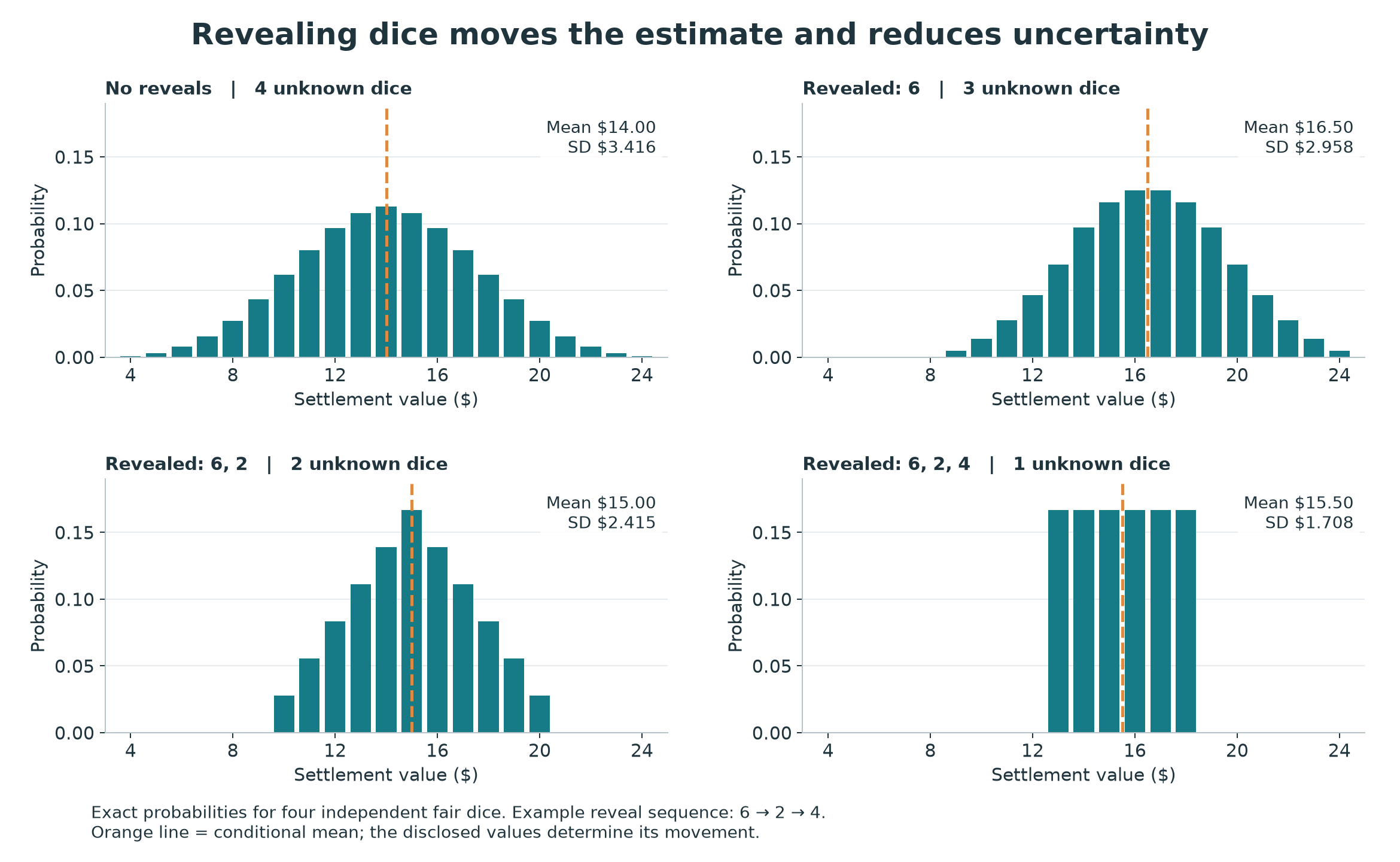
Four exact conditional payoff distributions for independent fair dice, with the example reveal sequence 6, 2, 4. Means move as values are revealed and standard deviations fall.

The example reveals are 6, then 2, then 4. Each panel uses exact probabilities; the orange line marks the conditional mean.

The mean can move up or down as values are revealed. In this independent-dice setup, the conditional variance falls by the same amount at each reveal, regardless of the revealed face.

The lower variance does not determine a particular spread. Inventory, customer information, and competition still matter. It tells us that remaining payoff uncertainty, one input to the quote, has changed.

Now hold five contracts on the same one-die outcome. Their settlement profit is

5V-15

, so:

\begin{aligned} \text{Var}(5V-15)&=25\text{Var}(V)=25\left(\frac{35}{12}\right),\\ \text{SD}(5V-15)&=5\sqrt{\frac{35}{12}}\approx8.539. \end{aligned}

The standard deviation grows fivefold because every contract shares the same payoff. Five independent die bets would be a different portfolio. The distinction is the same covariance issue we encountered in the linear algebra series.

Put volatility on the correct clock

Our earlier articles used annual volatility of 20%. A market maker may care about price movement over the next second or minute.

Suppose, purely for illustration, a stock has annual return volatility of 20%. Assume variance accumulates at a constant rate and increments are uncorrelated. Use 252 trading days and 390 minutes per day. Under these assumptions:

\begin{aligned} \sigma_{\text{day}}&\approx\frac{0.20}{\sqrt{252}}\approx1.26\%,\\ \sigma_{\text{minute}}&\approx\frac{0.20}{\sqrt{252\cdot390}}\approx0.0638\%. \end{aligned}

At a price of $100, that minute-scale return standard deviation corresponds approximately to a price standard deviation of $0.0638.

Holding 1,000 shares would give an approximate one-minute marked-profit standard deviation of $63.80 under those assumptions.

This conversion depends on the model. Actual intraday volatility varies with time and market conditions. Annual volatility estimated from daily returns includes risks that may not scale evenly across intraday minutes.

The square-root rule applies when variance grows in proportion to elapsed time. Brownian motion is a formal model with that property. At very short horizons, discreteness, bid-ask effects, and dependence also matter.

Keep two quantities distinct when writing code: return volatility, measured as a fraction, and price volatility, measured in dollars. For small price moves, multiply return standard deviation by the current price to approximate price standard deviation.

How likely is a trade?

Suppose a wider quote earns more per trade but attracts fewer customers. We need a model for the rate of fills.

A simple assumed relationship is:

\lambda(\delta)=A e^{-k\delta}.

Here, $\delta$ measures the quote’s distance from a reference price, in dollars. The parameter $A$ is a rate, such as fills per minute. The parameter $k$ controls how quickly that rate falls as distance increases. The units of $k$ are inverse dollars.

This is a modelling choice, not a law of markets.

If fills follow a Poisson process with fixed rate

\lambda

, the probability of at least one fill over a period of length

h

is:

\mathbb{P}(N_h\ge1)=1-e^{-\lambda h}.

At two fills per minute, the model gives $1-e^{-2}\approx86.5\%$ over one minute. Over one second, use $h=1/60$ , giving approximately 3.28%.

Multiplying a per-minute rate by 60 seconds without converting units would give the wrong result.

In a real order book, fills depend on order size, queue position, and incoming orders on the opposite side. Cancelling or revising your order also changes its chance of filling. Counts may cluster rather than follow a constant-rate Poisson model.

Turn the trade-off into an optimisation problem

Ignore inventory and information for a moment. Suppose every fill earns $\delta$ , and the expected fill rate is $Ae^{-k\delta}$ .

Expected earnings per unit of time are:

G(\delta)=A\delta e^{-k\delta}.

Using differentiation, we obtain:

G'(\delta)=Ae^{-k\delta}(1-k\delta).

For $A>0$ , $k>0$ , and $\delta\ge0$ , the maximum occurs at $\delta=1/k$ . If $k=100$ per dollar, that is one cent from the reference price.

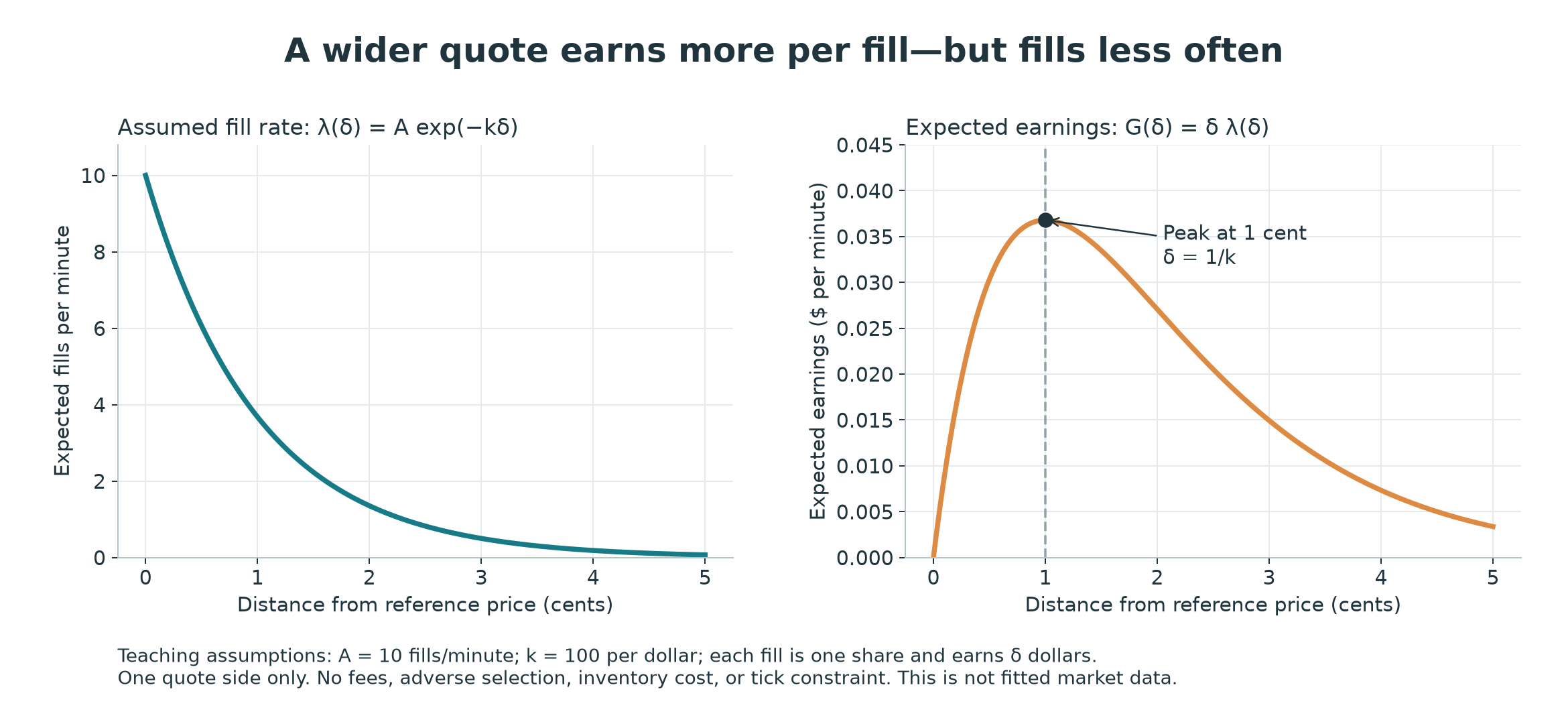
An assumed exponential fill rate decreases with quote distance while expected earnings peak at a one-cent distance, for the stated teaching parameters.

An illustrative one-share fill model with $A=10$ fills per minute and $k=100$ per dollar. The earnings curve covers one quote side and excludes costs and inventory risk.

The result shows how margin and fill rate interact under the stated assumptions. It does not tell us to quote a one-cent half-spread in an actual stock. Adding fees, conditional price moves, inventory penalties, and a minimum tick changes the problem.

For inventory, one transparent teaching rule is:

c_t=m_t-\eta q_t,\qquad b_t=c_t-d,\qquad a_t=c_t+d.

Here, $m_t$ is the observed midpoint, $q_t$ is inventory in shares, $\eta$ is a price shift per share, and $d$ is a half-width. A positive inventory shifts both quotes down. A negative inventory shifts them up.

With $\eta=0.001$ dollars per share, owning 10 shares lowers the quote centre by one cent. We choose this parameter to illustrate the policy. We have not estimated an optimal strategy. It is the policy we will experiment with in Part 3.

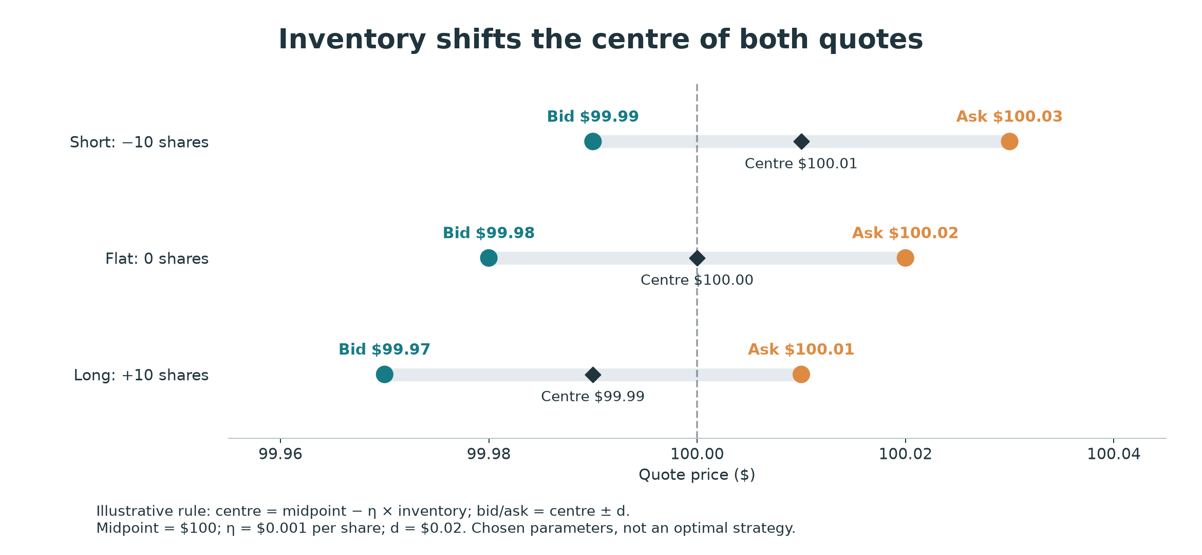
Bid, quote centre, and ask for short, flat, and long inventories under a chosen linear inventory rule. Long inventory lowers both quotes and short inventory raises both.

At a $100 midpoint, the chosen rule shifts the centre by one cent for ten shares of inventory. The two-cent half-width stays constant.

More formal models choose prices by balancing execution opportunities against inventory risk. Avellaneda and Stoikov's High-frequency trading in a limit order book is a useful advanced reference: it models price uncertainty, inventory preferences, and order arrivals to study quote placement. Study the assumptions before trying to calibrate the model.

Connect this back to linear algebra

For a single instrument, inventory is one number. With several instruments, it becomes a vector.

Suppose

q

contains positions in shares or contracts and

\Sigma_h

is the covariance matrix of their price changes, in compatible units, over horizon

h

. The variance of the marked position change is:

\text{Var}(\Delta\text{P\&L})=q^\top\Sigma_h q.

This has the same form as the portfolio-variance calculation, but the units have changed. We are using positions and price changes, rather than portfolio weights and percentage returns. Include each contract’s multiplier when calculating its exposure.

Vectors and linear combinations help organise exposures and hedges. Least squares can fit an imperfect relationship between observed features and later outcomes. Check the fit on later data before using it to make trading decisions.

The calculations follow a clear order. Use expectation to estimate value and conditioning to update it. Use variance to measure exposure. Then model fill arrivals and compare quoting policies.

Try the free SelfMadeQuant.com Market Making game again. Before each quote, calculate your expected sum and the number of unrevealed items. Then look at your current inventory. Explain why you chose the centre, width, and size separately. A free account lets you continue through settlement.

In Part 3, we will move from dice to public stock-market data. We will calculate spreads, measure what happens after actual trades, build a small database, and compare two hypothetical quoting rules in Python.

Until then, peace.