Quant finance projects for beginners: nine builds and what to learn first

Published 13 October 2026Updated 15 October 20267 min readBuild a quant project portfolio:Part 1Part 2 Part 3

A useful first quant finance project answers one financial question, produces a result you can check, and makes its assumptions visible. Good starting choices include an option calculator, a bond-risk explorer, a portfolio-risk dashboard, a small backtester or an order-book cost calculator.

The right choice depends on the work you want to investigate and the foundations you already understand. A volatility surface is a poor first assignment if you cannot yet explain an option payoff. A backtest becomes more useful once you can reconstruct its cash and positions by hand.

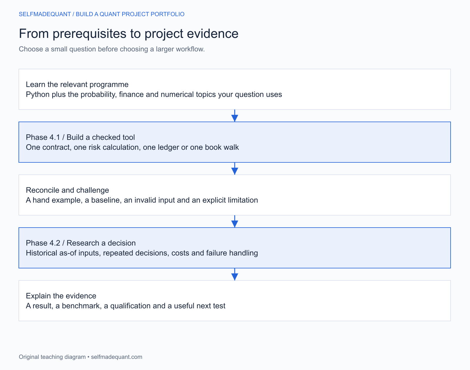
SelfmadeQuant’s project library has two levels. Phase 4.1 quick wins isolate a manageable calculation or investigation. Phase 4.2 applied research capstones extend that work into repeated decisions with historical data, benchmarks and controls. This guide maps the existing projects to prerequisite programmes so you can choose a route you can explain.

Browse Phase 4.1 quick wins and Phase 4.2 capstones in the public curriculum. Individual project links below open the app’s project workspace and follow its usual login and membership access.

A project learning pathway moves from prerequisite programmes to a checked Phase 4.1 tool and then a Phase 4.2 research workflow with evidence and limitations

Start with the programme that repairs your actual gap

Most routes benefit from Python for Quantitative Finance. If functions, arrays and tabular data are new, begin with the Python and Data Primer and the beginner Python guide.

For the mathematics, use Probability, Statistics and Financial Data when the project involves uncertainty, and Linear Algebra, Optimisation and Numerical Methods when it involves covariance, sensitivities or numerical solvers. Financial Instruments, Markets and Conventions supplies the contract and market vocabulary.

You do not need to finish every programme before touching a project. Start when you can explain the particular inputs and calculation, then return to the relevant lessons when a check exposes a gap. These are recommended preparation routes, rather than a claim that every listed programme is a formal access prerequisite.

Nine existing projects and their prerequisite programmes

Q1: European option price and Greeks calculator

Question: what does the chosen model price, and how does that value change when an input moves?

Open Q1 — Option Pricing and Greeks. Study Derivatives Pricing and Computational Finance alongside it, particularly payoffs, discounting and the Black–Scholes assumptions. Probability and basic differentiation support the formula and sensitivities.

Your first deliverable is a European call-and-put calculator with explicit maturity, rate, dividend and volatility units. Check put–call parity and compare analytic delta with a finite-difference calculation. Expiry and zero volatility need deliberate treatment.

The reference project also examines a frozen BTC option snapshot. That extension investigates model limitations; it does not make a single constant-volatility price the correct mark for every quoted option. Continue toward the OV pricing-control capstone when you can reconcile the calculator before introducing real quote conventions.

Q2: volatility smile and surface explorer

Question: how does implied volatility vary across strikes and maturities, and which quotes or interpolated values are inconsistent?

Open Q2 — Volatility Smile and Surface after Q1. The main preparation is the Options Pricing programme, with numerical interpolation from Linear Algebra, Optimisation and Numerical Methods.

Begin with a small labelled grid. Reproduce the input nodes, reject duplicate coordinates, and identify unsupported extrapolation. Then examine call-price monotonicity and convexity. A smooth image is not evidence that the implied prices are arbitrage-free.

This route also leads to OV. The progression is from plotting a surface to deciding which observed quotes support a valuation and how a rejected quote changes that decision.

Q3: bond price, duration and DV01 explorer

Question: how much does a bond lose when yields move, and what remains after a simple hedge?

Open Q3 — Bond Duration and DV01. Prepare with Fixed Income and Interest-Rate Models, supported by cash-flow discounting and derivatives.

Start with a fixed-rate bullet bond under one stated settlement and compounding convention. Check a par bond, a zero-coupon bond and the sign of the price response to a yield rise. Compare exact repricing with duration and convexity approximations.

A DV01-matched hedge offsets a specified small parallel move; it does not neutralise every change in curve shape. That limitation provides the bridge to TR — Treasury Curve Risk and Hedge Validation, where key-rate exposures and repeated hedge reviews become central.

Q4: portfolio risk and diversification dashboard

Question: which holdings contribute to portfolio risk, rather than merely receive the most capital?

Open Q4 — Portfolio Risk and Diversification. Prepare with Portfolio Theory and Quantitative Investment and the Linear Algebra programme.

Calculate portfolio volatility from a covariance matrix and reconcile it with the volatility of the weighted return series under the same constant-weight convention. Then decompose the total into risk contributions.

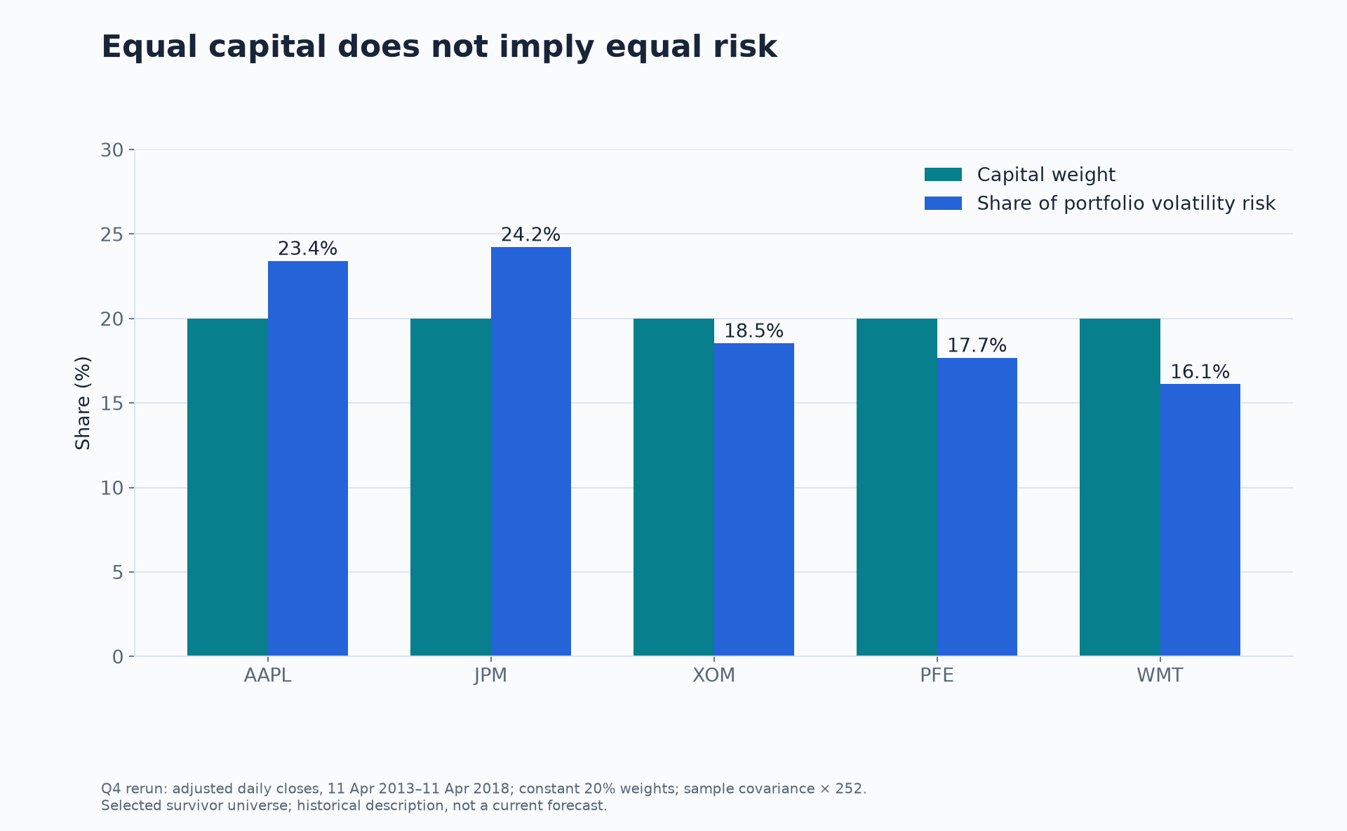
The existing five-stock example gives every asset 20% of capital, but JPM contributes about 24.2% of volatility risk and WMT about 16.1%. The chart below reproduces that calculation on the frozen 2013–2018 window. The selected historical stock universe has a survivorship limitation; these percentages are not current risk estimates.

Recomputed risk contributions for the existing five-stock Q4 example differ from its equal 20 percent capital weights, with JPM near 24.2 percent and WMT near 16.1 percent

Extend this route through PR — Portfolio Risk Forecasting and Rebalancing Control once you are ready to test changing weights, future realised risk and implementation costs.

Q5: drawdown and tail-loss monitor

Question: how large were losses, and does a simple risk estimate describe their frequency and severity adequately?

Open Q5 — Drawdown and Tail-Loss Monitor. Prepare with Quantitative Risk Management and Probability and Statistics.

Build a wealth index, measure drawdown from its previous peak, and compare historical and model-based tail estimates. State whether a displayed loss is a positive magnitude or a negative return. A correct aggregate breach count can still hide clustering.

Continue to VR — Volatility Forecasting and Risk Limits when you want to turn next-day risk estimates into an exposure decision. Add Econometrics and Financial Time Series before comparing dynamic forecasts.

Q6: minimal strategy backtester

Question: does the reported strategy result follow from feasible signals, fills and accounting?

Open Q6 — Strategy Backtester. Prepare with Quantitative Research, Data and Backtesting and the Python programme.

Start with a tiny ledger whose final cash you can calculate independently. A signal formed after today’s close should not receive a fill at an earlier price. Include fees, initial positions and terminal liquidation consistently for the strategy and benchmark.

The reference implementation shows why a striking equity curve can depend on a pre-window position and a selected starting date. Its transferable skill is timing and accounting, with routes toward PR and EX. For the implementation method itself, use how to backtest a trading strategy in Python.

Q7: Monte Carlo pricing and convergence lab

Question: is the estimated price accurate enough, and does its reported error bar behave as expected?

Open Q7 — Monte Carlo Convergence. Prepare with the Options Pricing and Probability and Statistics programmes. Q1 supplies an analytic benchmark for a compatible European contract.

Vary the simulation budget, use independent replications and check interval coverage. Sampling precision, contractual monitoring and model uncertainty are different questions. Antithetic sampling should be checked for the actual payoff rather than enabled on the assumption that it always helps.

Continue to OV for pricing-model control or IV for independent validation. The Monte Carlo option-pricing article supplies a smaller worked introduction before the project workspace.

Q8: order-book and slippage calculator

Question: what would a specified marketable order cost against the displayed liquidity?

Open Q8 — Order-Book Slippage. Prepare with Market Microstructure and Execution and the instruments programme.

Walk an order through successive levels, calculate the volume-weighted price, and keep fees separate from book impact. Quantity beyond the observed depth must remain unfilled unless you introduce and label an additional execution assumption.

This is the natural starting point for EX — Execution Replay and Transaction-Cost Diagnostics and MM — Inventory-Aware Market-Making Research. A static snapshot cannot establish how a hypothetical order would change other traders’ behaviour or where a resting limit order would sit in the queue.

Q9: Bitcoin event-probability explorer

Question: what do a simple model, option-implied information and an event quote say about the same specified event?

Open Q9 — BTC Probability Explorer. Prepare with Probability and Statistics, Options Pricing and the relevant market-convention lessons.

Define the event, observation time and settlement rule before comparing numbers. The reference project’s prediction-market contract and quotes are illustrative: the intended live source was geographically unavailable during acquisition. That part is not a completed real-market comparison.

A physical probability and a price-implied probability can differ for reasons other than a tradeable opportunity. Treat this as a probability and data-definition investigation, with the unavailable source explicitly recorded.

Choose one route, then a second complementary check

For pricing, start with Q1, then add Q7’s numerical validation or Q2’s quote diagnostics. For portfolio work, start with Q4 and use Q6 to learn the accounting behind changing allocations. For execution, start with Q8 and use Q6’s timing discipline before replaying a schedule. For rates, Q3 gives a direct route to TR; for risk, Q5 gives a direct route to VR.

Those are suggested pairings, not a requirement to complete all nine. The complete beginner quant roadmap remains the destination for your overall study sequence. This page answers the narrower question of which project to build.

Decide what “finished” means before adding an interface

A first project is ready to explain when someone else can identify its inputs, run its baseline, reproduce an independently checked example and see a meaningful failure case. A calculator should reject an invalid input clearly. An empirical comparison should state the sample, benchmark and limitations next to the result.

Keep the calculation separate from its presentation. A notebook, small script or local tool can be sufficient. A web interface adds value when it helps the reader inspect the financial question; it does not replace the numerical checks.

Write a short note answering: what did I calculate, what assumption mattered most, and what would change the conclusion? Then move to building a quant research project or presenting the evidence in an interview.

Open the project with the preparation beside it

Use the public project catalogue to compare scope, data and outputs. In the app, the project workspace provides its overview, report, notebook and available files. Follow that project’s reproduction instructions; quick wins and capstones use different workspaces and dependencies.

If a prerequisite is missing, repair that specific gap in the linked programme. The foundation code resources provide small standalone examples before you attempt a full project.