How to build a quant research project: from a quick win to a role capstone

Published 15 October 20268 min readBuild a quant project portfolio:Part 1Part 2Part 3

To build a quant research project, start with a decision, establish a simple checked baseline, freeze the information available at each historical date, and evaluate what happens when the decision is repeated. Finish with a reproducible report that distinguishes observed data, model assumptions and unresolved limitations.

A working formula is an important first stage. A research project adds evidence about when the tool is useful, how it fails and whether a more complicated method improves the actual decision. The change from a small notebook to a capstone is therefore a change in the question and validation, as well as in the amount of code.

SelfmadeQuant’s Phase 4.1 quick wins and Phase 4.2 capstones make that progression concrete. This article follows portfolio, execution and pricing routes through existing projects, then maps the other implemented capstones to their preparation.

If you are still choosing a starting calculation, use the quant project ideas guide. This page focuses on research design rather than duplicating the implementation tutorials.

Write a decision question with a benchmark

“Can I optimise a portfolio?” is too broad to evaluate. “Does a constrained minimum-variance allocation reduce future realised risk relative to equal weights after a stated rebalance policy?” identifies the decision, comparison and outcome.

“Can I build an execution algorithm?” becomes more useful as “Does slicing this order improve the cost-risk trade-off relative to immediate execution under the same fees and information?” The benchmark belongs in the question before you inspect which method wins.

Write a short protocol covering the universe, observation dates, decision frequency, available inputs, benchmark, evaluation metric and conditions that would count against your preferred method. If you change it after seeing results, record the change. A polished final report should not erase the sequence of experiments that produced it.

A research workflow turns a checked calculation into an as-of input snapshot, a recorded decision, an outcome and a monitored exception

Route 1: portfolio risk becomes a rebalance decision

Start: Q4 — Portfolio Risk. Add accounting: Q6 — Strategy Backtester. Progress to: PR — Portfolio Risk Forecasting and Rebalancing.

The prerequisite sequence is Linear Algebra, Optimisation and Numerical Methods, Portfolio Theory and Quantitative Investment, and Quantitative Research, Data and Backtesting, supported by Python. The programme outcomes matter more than treating the list as a box-ticking exercise.

Q4 establishes a snapshot calculation. For fixed weights and a consistently estimated covariance matrix,

\sigma_p=\sqrt{w^\top\Sigma w},\qquad RC_i=\frac{w_i(\Sigma w)_i}{\sigma_p},\qquad \sum_i RC_i=\sigma_p

when portfolio volatility is positive. That identity is a numerical check; it does not tell you which future covariance estimate will work best.

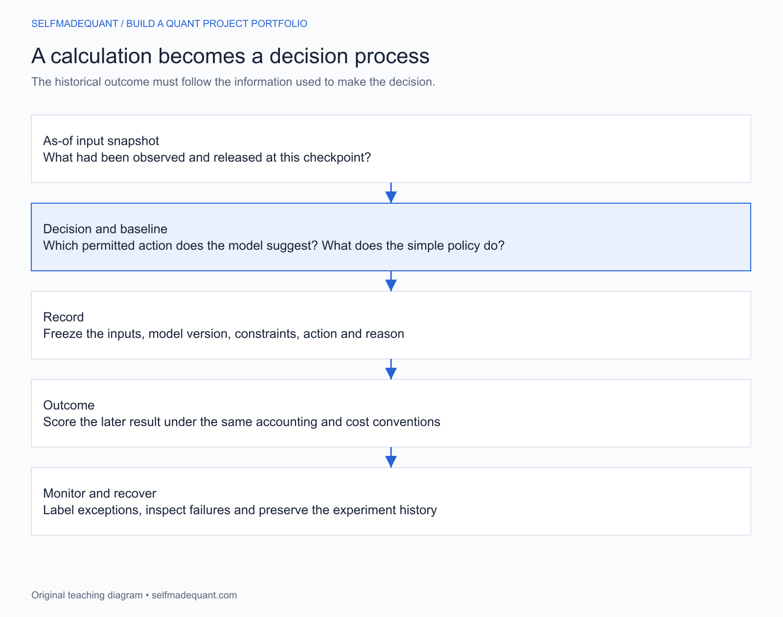
PR adds model comparison, a changing investable book, distributions and splits, constraints, approvals, assumed trading costs and a decision ledger. It asks what should be traded at a particular month end using information available then, and what risk and return follow.

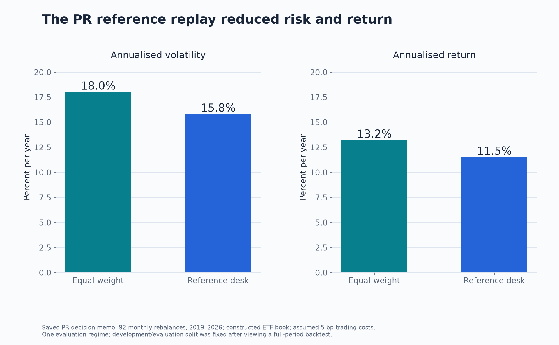
The reference desk replay reports annualised volatility of 15.8% versus 18.0% for equal weights, but annualised return of 11.5% versus 13.2%, after its assumed five-basis-point trading costs. Lower risk did not establish a return improvement.

Saved PR reference replay results show lower volatility and lower return than equal weight; the chart separates the two annual percentage measures

These figures summarise the existing historical reference report; they are not a newly rerun capstone or live performance. The study uses a constructed sector-ETF book and one evaluation regime. Its report also discloses that the development/evaluation split was fixed after a full-period backtest had been seen. The conclusion needs that qualification.

The valuable extension is an explanation: which sectors and constraints caused the gap, did the covariance method add measurable value, and what would invalidate the result? Copying the lower-volatility number into a headline would leave most of the research unfinished.

A useful failure drill is an infeasible constraint. Eleven fully invested, nonnegative weights cannot each be capped at 8%, because their maximum total is 88%. A system should identify that before trusting an optimiser’s output. The PR reference includes this kind of explicitly injected control test.

Route 2: a book walk becomes an execution replay

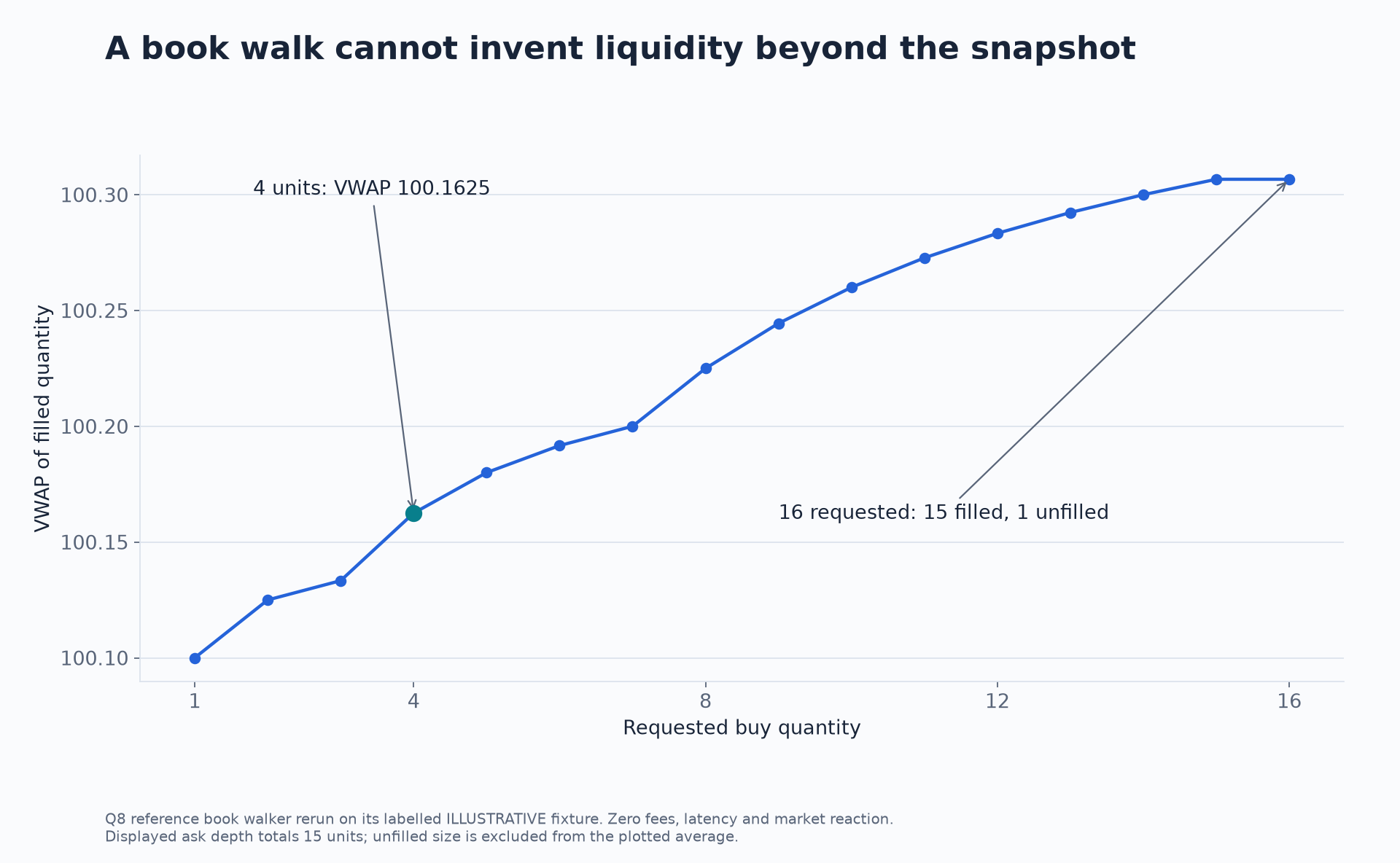
Start: Q8 — Order-Book Slippage. Progress to: EX — Execution Replay and Transaction-Cost Diagnostics. For quoting and inventory, choose MM — Inventory-Aware Market Making instead.

Prepare with Market Microstructure and Execution, Probability and Statistics and the relevant research and data-engineering topics. EX is about working a parent order; MM is about posting quotes and managing inventory. They share data infrastructure but answer different decisions.

In Q8’s illustrative book, buying four units takes one at 100.10, two at 100.15 and one at 100.25. The average is

\mathrm{VWAP}=\frac{100.10+2(100.15)+100.25}{4}=100.1625.

The midpoint is 100.05, so impact is approximately 11.24 basis points. Fees are separate. Fifteen units exhaust the displayed ask depth; requesting sixteen leaves one unfilled. These are checks on a labelled artificial snapshot, not market observations.

The actual Q8 reference book walker on its illustrative fixture shows increasing average execution price as size grows and leaves quantity beyond fifteen units unfilled

EX then rebuilds historical book updates, defines order arrival and child-order timing, compares schedules, stresses latency and records what happens when the feed is invalid. Its reference study uses 69 first-of-month Coinbase sessions, rather than continuous coverage of every day in the period.

The study found that a lower average slicing cost came with substantial price-risk dispersion, while the assumed fee exceeded the impact cost of each order size studied. That is a finding about its historical sample, order sizes and replay assumptions. It is not a universal instruction to send every order immediately.

The missing counterfactual is unavoidable: the recorded market did not react to the hypothetical orders. A replay can reconstruct observed depth and impose optimistic/conservative assumptions; it cannot reveal the exact alternative market path those orders would have created.

For the feed mechanics, Coinbase’s WebSocket documentation is a primary reference. The project provides its own acquisition and reconstruction contract. Confirm which channel and sequence rules your implementation actually uses before treating messages as a valid book.

Route 3: a price becomes a valuation-control decision

Start: Q1 — Option Pricing and Greeks, then Q2 — Volatility Surface and Q7 — Monte Carlo Convergence. Progress to: OV — Option Quote Validation and Pricing Control.

Prepare with Derivatives Pricing and Computational Finance, the probability and numerical-methods programmes, then the relevant Advanced Derivatives and Exotic Options material. Start with a contract you can price independently before tackling a full quote-control workflow.

Q1 verifies a formula under explicit assumptions. Q2 examines consistency across quotes. Q7 separates simulation error from monitoring and model choices. OV combines quote selection, valuation, uncertainty, sensitivity reconciliation and exception handling over repeated historical checkpoints.

The existing OV report illustrates a subtle result: the constrained surface met the relevant no-arbitrage checks, yet its held-out quote fit was worse than simple interpolation in that experiment. Structural validity and predictive fit are different evaluation criteria. Neither a smooth surface nor a more elaborate model earns automatic preference.

The capstone also uses inverse, coin-margined contracts. Payoff, settlement and numeraire conventions must be checked before reusing a cash-equity formula. Use the project’s contract specification rather than assuming that the word “option” makes every input interchangeable.

Gatheral and Jacquier’s arbitrage-free SVI paper supplies one of the project’s research foundations. The project report supplies the actual study design and the limits of its comparison. Read both before extending the implementation.

Other implemented capstones and the preparation they need

The live project catalogue checked for this guide contains nine quick wins and ten capstones. The following routes complement the four capstones linked above. The quick win supplies a component skill, rather than all the domain knowledge required for the larger project.

Phase 4.2 project	Useful Phase 4.1 preparation	Main prerequisite programmes
TR — Treasury curve risk and hedge validation	Q3 bond pricing and sensitivity checks	Fixed Income, Linear Algebra and Numerical Methods
VR — Volatility forecasting and risk limits	Q5 tail-loss monitoring	Econometrics, Quantitative Risk Management
MV — Real-time macro forecasting	Q6 information timing; macroeconomics is additional preparation	Econometrics, Research and Backtesting
FD — Filing change and deterioration monitor	Q6 timestamp discipline; filing analysis is additional preparation	Text as Data and NLP, Research and Backtesting
AL — Deposit betas and balance-sheet risk	Q3 repricing intuition; deposit modelling is additional preparation	Fixed Income, Risk Management, Instruments and Conventions
IV — Independent model validation and change control	Q7 numerical validation and Q5 loss measures	Risk Management, Professional Quant Practice

The earlier planning documents also describe mortgage and systematic-signal capstones. They were not in the live implemented project catalogue checked for this article, so they are not presented here as available workspaces. Check the current catalogue as the library develops.

Make the data contract part of the research

For every input, record its source, units, observation time, availability time and revision policy. A value observed for March may not have been published in March. A later revised economic series is not automatically what a researcher knew at the historical decision date.

Use immutable snapshots or versioned files so the baseline can be reproduced. Hash checking establishes that the input bytes have not changed; it does not prove those bytes are economically correct. Include domain checks for splits, missing data, stale quotes and implausible conventions.

External data are useful only after their definitions are understood. The Kenneth French Data Library supports research-return comparisons, while the Federal Reserve’s nominal yield-curve data support rates research. Neither source alone supplies an executable trading strategy, a complete security ledger or every required availability timestamp.

Add one meaningful extension and one failure drill

Choose an extension that tests a claim: a changed covariance window, a cost sensitivity, a held-out strike or a different execution latency. Keep the baseline visible. Adding a second library that calculates the same quantity without an independent check provides little new evidence.

Then inject one labelled failure. Make a constraint infeasible, delay a data release, remove a required quote or interrupt a replay. Record whether the system rejects the input, holds the previous decision or uses a documented fallback. Quietly filling missing values or inventing a fill changes the experiment.

Finish with the outcome, benchmark difference, uncertainty and limitation in one short memo. If the new method fails, explain what the failed comparison taught you. That is a complete research result when the question and evaluation were sound.

Open the existing workspace and build the next stage

Choose a route in the project catalogue, open its prerequisite programme beside it, and follow that project’s run instructions and access conditions. The existing workspace is the place for its full notebook and files.

For a worked code introduction, use the existing backtesting guide, Monte Carlo pricing guide or portfolio rebalancing guide. When you can explain the decision and the evidence, continue to presenting a quant project in an interview.