How to backtest a trading strategy in Python: start with the cash

Published 13 October 20265 min readBacktesting and strategy evaluation:Part 1Part 2 Part 3 Part 4 Part 5

You have a trading rule. Buy when the price moves above its recent average. Sell when it falls below.

You run it through a spreadsheet. The line goes up. Then someone asks when you placed the orders, what prices you received, and whether the cash account ever went negative.

Those questions decide what the line means.

A backtest applies a specified decision rule to past observations, under explicit assumptions about information, execution and accounting. It tells you what that simulated process would have produced on that sample. To interpret it, you need to reconstruct the decisions and the money.

In this series we will build one small Python experiment, deliberately break its timing, introduce costs, select parameters using earlier observations, and report what survives. The aim is a result another person can inspect.

Write the trading contract before the code

Our teaching asset has an opening price and a closing price for each numbered session. It pays no dividends. We can hold fractional shares or cash, with no borrowing, shorting or leverage. Cash earns zero interest.

At each completed close, compare that price with the average of the last 20 closes, including the close just observed. If it is above the average, request a fully invested position at the next session's open. Otherwise request cash.

Remain invested until the rule changes. We do not sell and repurchase every day merely because a fresh signal arrives.

At the final session's close we liquidate any shares. That terminal liquidation is part of the protocol written before running the experiment. Charge costs on entry and exit, including this final sale.

Decision	Our assumption
Information	Only completed closes, observed before the next opening trade
Signal	Close above its trailing 20-session mean
Execution	Next observed open, with a specified proportional cost
Position	Either fully invested or cash; no daily rebalancing while invested
Initial wealth	$100,000
Evaluation	Sessions 80 through 1511 inclusive
Terminal position	Cash after the predeclared final-close liquidation

The opening price is a teaching execution proxy. A live order needs an arrival time, order type, available liquidity and a defensible fill model. Daily bars alone cannot establish those details.

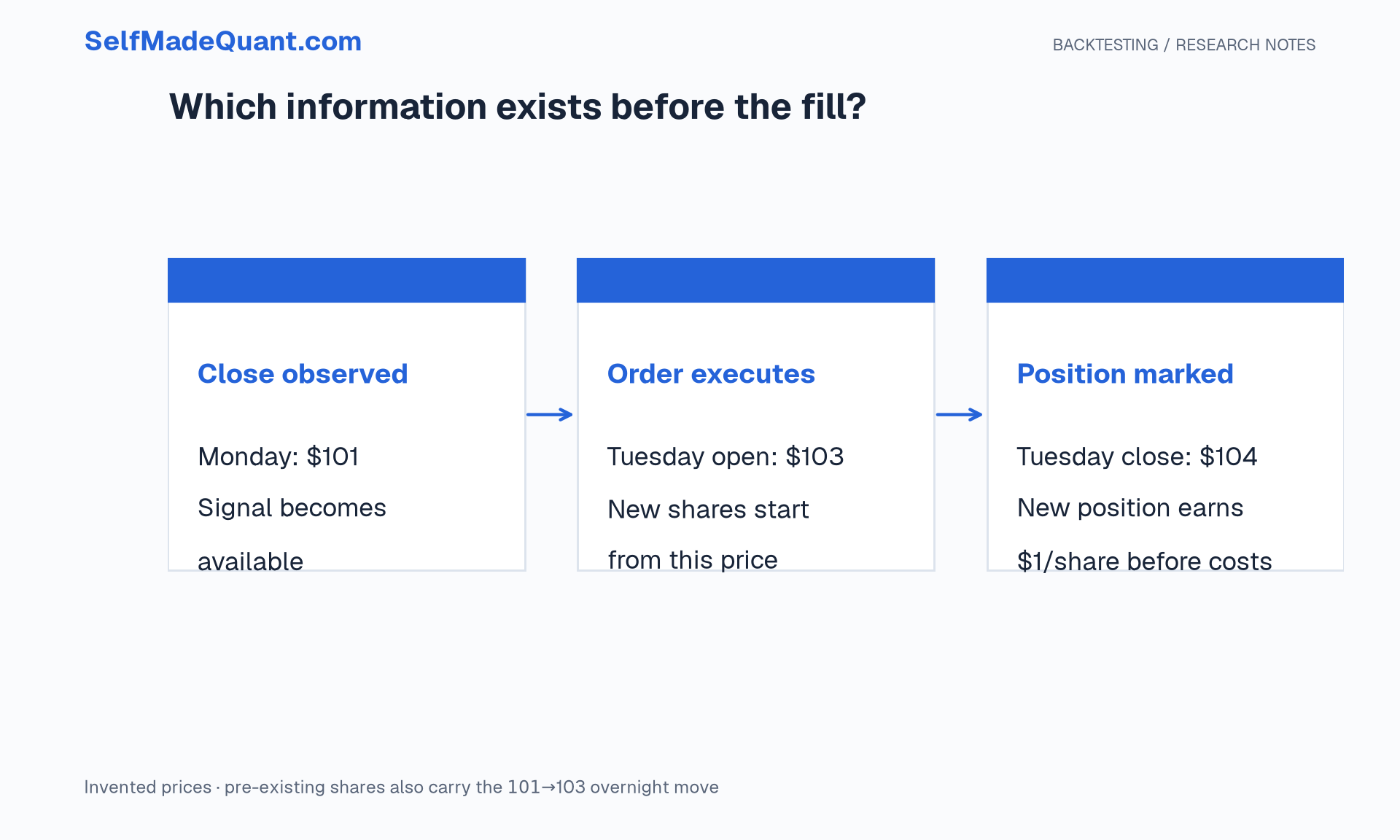
A completed closing observation creates an order for the following opening session

The information used by the signal precedes the simulated opening fill. An existing position also carries overnight risk.

Keep signal time and return time separate

Suppose Monday closes at $101, above its trailing mean. The signal is known after Monday's close. Tuesday opens at$ 103 and closes at $104.

An order executed Tuesday at $103 earns one dollar per share by Tuesday's close. It does not earn the two-dollar gap from Monday's$ 101 close to Tuesday's $103 open if we were previously in cash.

If we already held shares from an earlier trade, those shares do earn or lose the overnight price change. The same price gap affects different portfolios differently because their starting holdings differ.

That is why blindly multiplying a signal by a close-to-close return can misstate this strategy's profit. The accounting must match the execution rule.

The signal itself is short:

import pandas as pd

def opening_target(close, window=20):
    mean = close.rolling(window, min_periods=window).mean()
    at_close = close > mean
    return at_close.shift(1, fill_value=False).astype(int)

example = pd.Series([100.0, 101.0, 102.0, 99.0])
print(opening_target(example, window=2).tolist())
# [0, 0, 1, 1]

The last target is still one because the preceding close was $102. The$ 99 close changes the following opening decision. A falling market is allowed to hurt the position before we can react.

Buy the shares you can actually afford

Let cash before an entry be B, the opening price be P, and the one-way proportional cost be c. Buying q shares requires qP for the asset and cqP for costs.

The affordable position is:

q=\frac{B}{P(1+c)}.

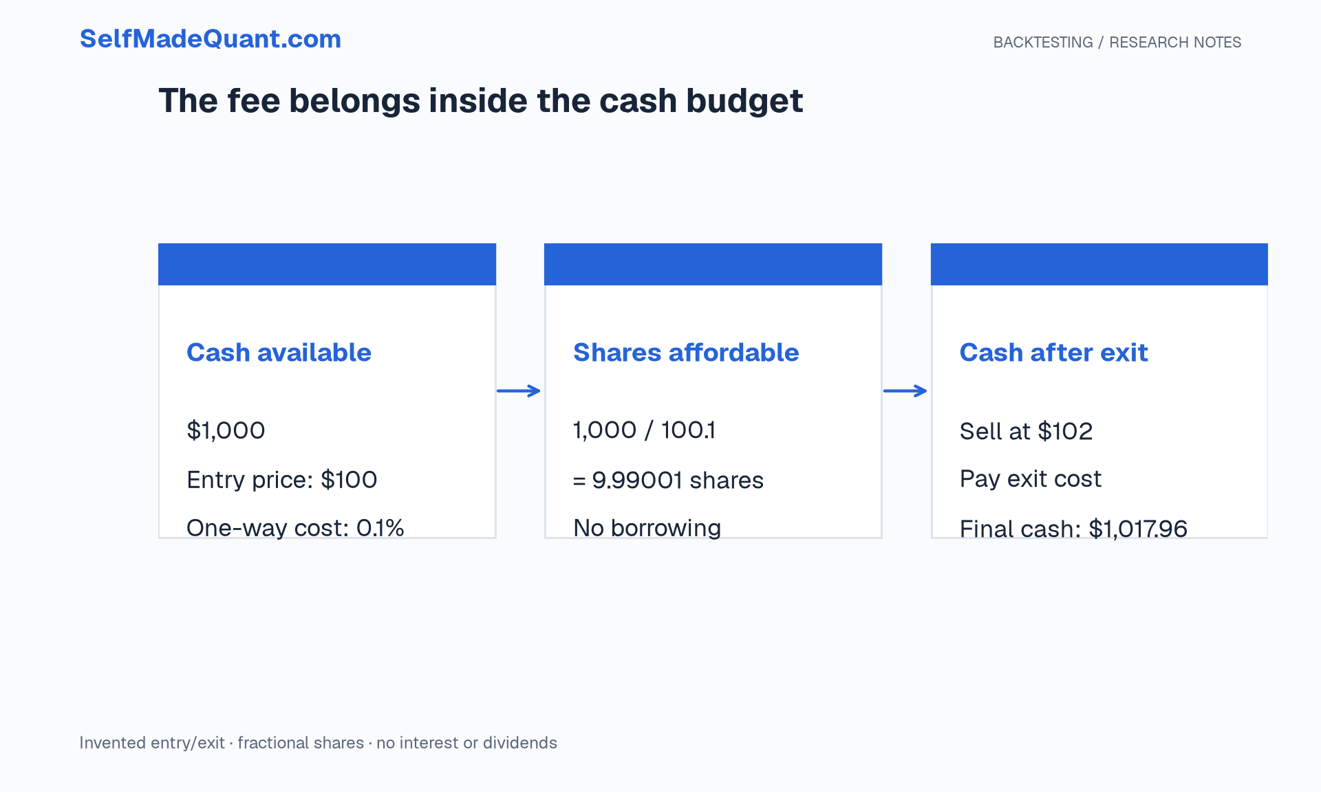
With $1,000, a$ 100 opening price and a 0.1% one-way cost, we buy approximately 9.99001 shares. Spending the full $1,000 on shares and charging another dollar would create an unintended negative cash balance.

Suppose the position is later sold for $102, with the same cost rate. Final cash is approximately$ 1,017.96. The gross price move was 2%; the account earned about 1.796% after both costs.

Marking those shares at an intermediate $110 close would show roughly$ 1,098.90 of wealth. If the next execution is $102, that temporary valuation is never realised as a sale at$ 110.

Reconcile every session

At each close, portfolio wealth is cash plus the marked value of the shares:

W_t=B_t+q_t C_t.

Break its change into the overnight gain on the shares brought into the session, the intraday gain on the shares held after the opening trade, and explicit trading costs. For a session without a terminal-close sale:

W_t-W_{t-1}=q_{t-1}(O_t-C_{t-1})+q_t(C_t-O_t)-K_t.

Here K is the dollar trading cost. On the predeclared terminal sale, use the shares held during the session for intraday profit, then set end-of-session holdings to zero and deduct the exit cost.

Our distributed ledger records cash, shares, wealth, gross profit, costs and turnover separately. It checks that wealth changes equal gross profit minus costs to numerical tolerance.

This is a useful invariant. It catches mistakes that a plausible equity chart can hide, such as charging costs twice or forgetting gains on an overnight position.

The ledger separates gross profit, costs and changes in wealth

A cost is a cash outflow. A price change affects the shares actually held during that interval.

Run the offline experiment

The reader package contains the full cash-and-shares implementation, fixture, ledgers and result tables. It generates 1,512 synthetic sessions with NumPy seed 42, then reloads the distributed CSV before calculating results.

Overnight and intraday log returns are independent normal draws with constant parameters. There is no deliberately embedded trend-prediction mechanism. The moving-average rule is a specimen for testing the machinery, rather than an established source of alpha.

Run from the package's lab directory:

from backtest import run

result = run()
print(round(result['fixed_window_cost_sensitivity']['5']['total_return'] * 100, 2))
# -7.49

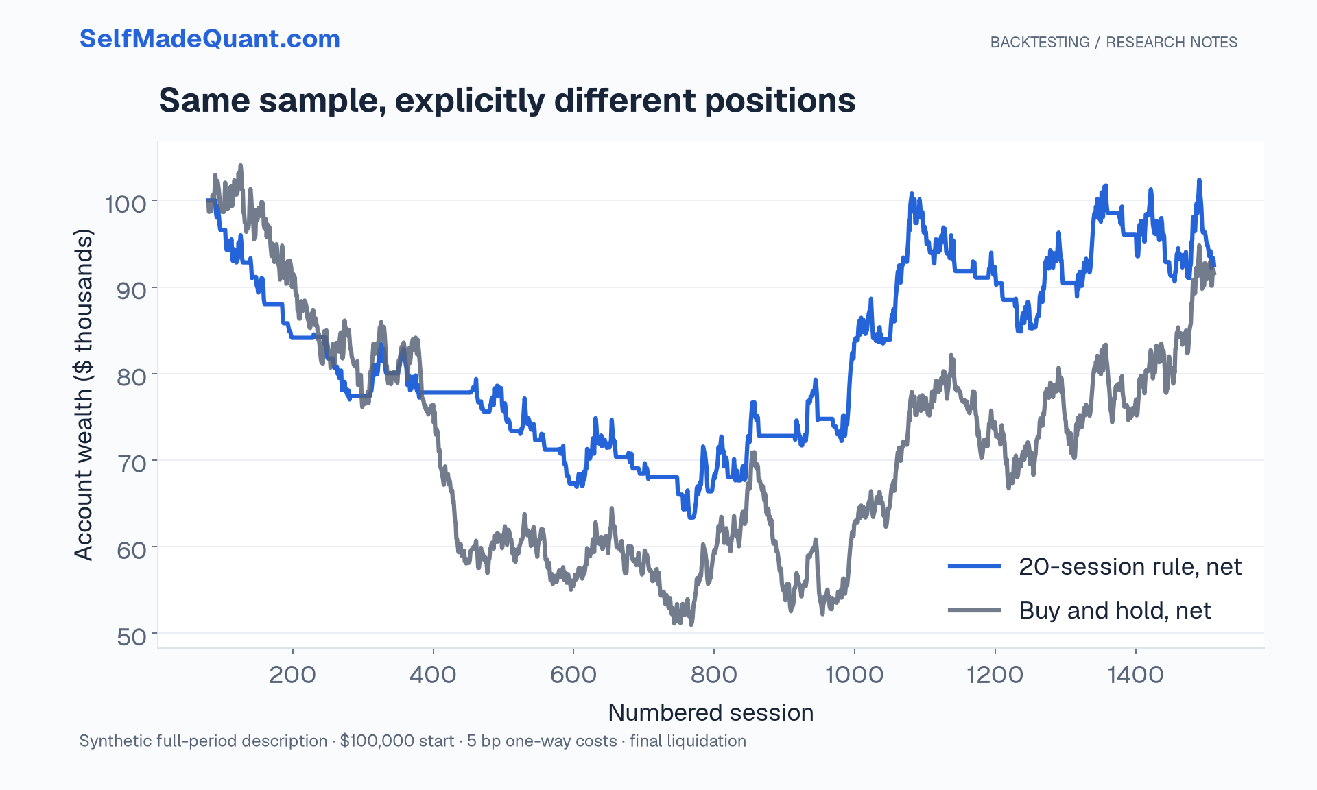
The fixed 20-session rule ends with $92,514.17 after the baseline 5 bp one-way cost. Before costs, the corresponding run ends with$ 101,125.45. Buy and hold, over the same evaluated sessions and with the same entry and exit cost rate, ends with $91,606.97.

The strategy has a slightly better terminal result than buy and hold in this sample, while both lose money. It spends roughly half its signal sessions invested, so the exposures also differ. Relative performance alone does not show predictive skill.

Synthetic strategy and buy-and-hold wealth over matching sessions

Seed 42, synthetic prices, $100,000 initial cash and 5 bp one-way costs. These full-sample curves describe the fixture; they are not a held-out test of a selected strategy.

What would change with real data?

Real instruments introduce distributions, corporate actions, changing constituents, trading calendars and data revisions. A split can look like a catastrophic return if you mix incompatible price conventions. A dividend changes the cash account even if a price-only chart misses it.

Record where each observation came from, its timestamp and its adjustment convention. If you use current index constituents throughout history, you can silently exclude securities that disappeared. QuantConnect's research guide discusses this survivorship problem and related research biases.

Our synthetic asset removes those data issues so that the accounting is visible. A future real-data implementation must put them back into the specification.

Before trusting a result, select one entry, one overnight holding and one exit. Reproduce their cash flows by hand. Then check the full ledger.

In the next article, we will use information from the wrong side of the execution time and watch the result improve for a reason that cannot be traded.

For the full series and runnable files, visit the backtesting resources. Subscribe separately to SelfMadeQuant on Substack for the next explanation.

Until then, peace.