Portfolio rebalancing in Python: test the weights you could have chosen

A minimum-variance allocation should minimise variance under its supplied covariance matrix. That does not promise a higher realised return, lower drawdown or lower future realised variance than every baseline. A useful experiment keeps those claims separate.

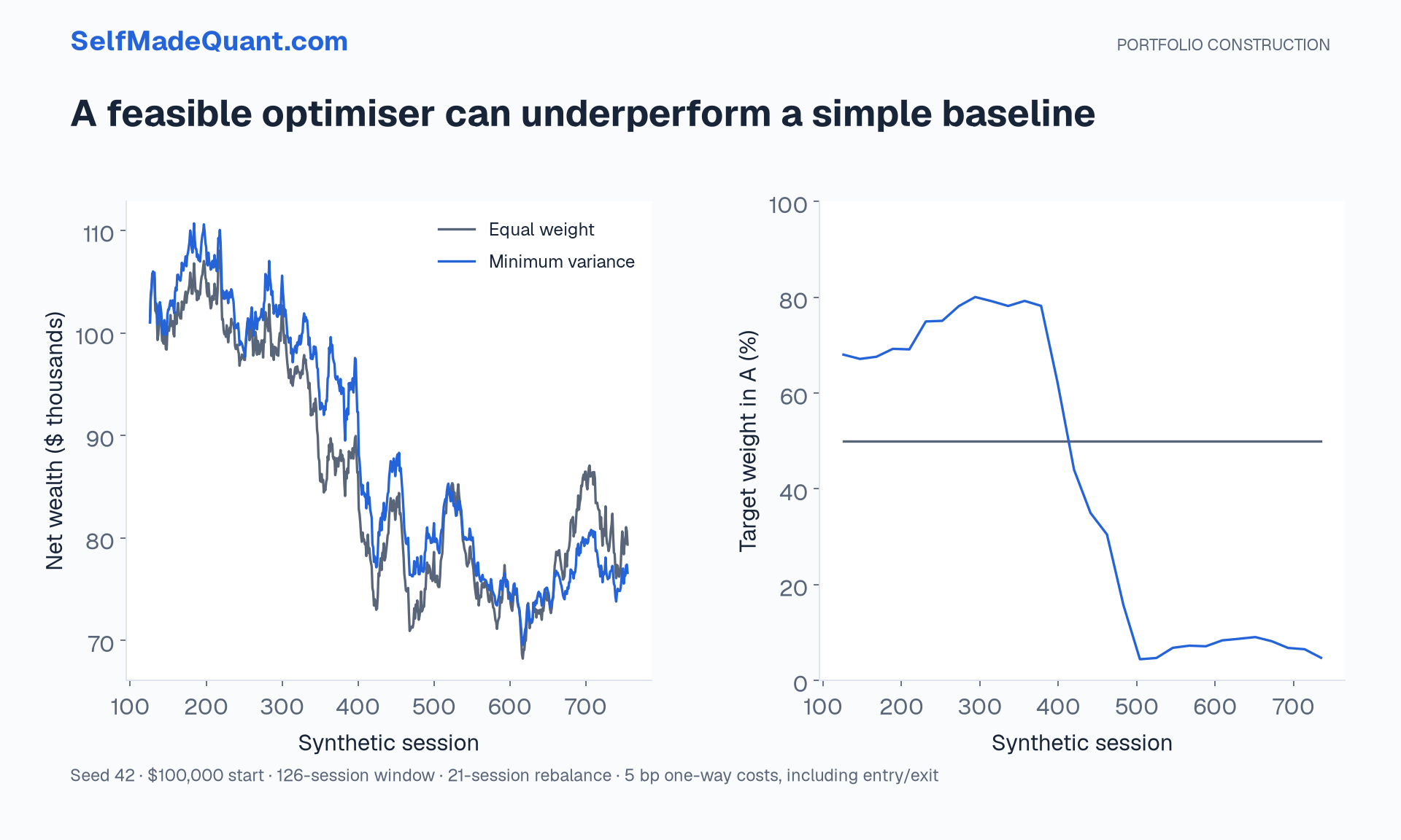
Our small Python lab compares equal weights with a rolling minimum-variance rule on two synthetic assets. The optimised rule ends with less wealth on this particular path. That result is useful because it prevents the optimiser's name from replacing an account-level evaluation.

The project uses only Python's standard library. Its purpose is inspectable timing, estimation and transaction accounting, rather than finding a profitable allocation.

Declare the experiment before generating the result

Generate 756 sessions using a seeded Gaussian teaching process, seed 42. The two assets' volatility and correlation parameters change at session 378. This is a deliberately specified regime change, not a claim that real returns follow this model.

The account begins investing at session 126 with capital of 100,000. The first 126 returns are estimation history only. Rebalance every 21 sessions, using the immediately preceding 126 returns. Cash earns no interest; shorting and leverage are excluded.

Equal weight targets 50/50 at every rebalance. Minimum variance estimates the two-asset sample covariance, blends it 50% towards its diagonal, and solves the fully invested long-only minimum. The lookback, rebalance interval and blend are fixed teaching choices, not parameters selected to maximise this run's performance.

Use only returns available before the trade

At decision session t, estimate covariance from rows t − 126 through t − 1. Choose the target before applying return t. The synthetic experiment assumes trading at the period boundary and then receiving that period's return.

There is no intraperiod execution model. Real data would require separate tradable prices, timing, market impact and availability evidence. The simulation's boundary convention makes the experiment well defined without pretending to measure those additional quantities.

The code records target weights separately from the holdings that drift after returns. On sessions without a rebalance, it carries those holdings forward. Reapplying the target daily would implement a different strategy.

Charge costs on the actual transactions

Every risky-asset purchase and sale pays five basis points of traded value. Entry and final liquidation are included. A change of weights consumes cash, so target holdings are fractions of wealth after paying the fee.

Let f be the transaction fee as a fraction of pretrade wealth, c the one-way rate, w the target risky weights and v the current risky weights. The self-financing fee equation is:

The lab solves this scalar equation by bisection, then applies the target weights to the remaining wealth. At initial entry, current risky weights are zero and the rest of the account is cash. Cash transfers themselves are not charged as a third asset trade.

This avoids charging a guessed turnover percentage while allocating the original wealth as though the fee never left the account. It remains a proportional-cost teaching model: the five-basis-point assumption is not measured execution evidence.

Inspect the result without changing the question

Equal weight finishes at 79,352.63, a return of −20.65%, with maximum drawdown of −36.84%. The rolling minimum-variance rule finishes at 76,595.13, a return of −23.40%, with maximum drawdown of −37.16%.

Total fees are 127.49 and 179.52 respectively. Traded dollars divided by initial capital are approximately 2.55 and 3.59. This turnover convention uses initial capital throughout; it differs from conventions that normalise each trade by contemporaneous wealth.

The account comparison includes entry and final closing fees. The maximum drawdown calculation uses the initial capital as its starting peak and includes final liquidation. Every printed statistic refers to the same defined account.

The optimised rule underperforms here. This does not disprove minimum-variance optimisation: the rule minimised its estimated variance at each decision. Nor would a better endpoint prove its superiority. A single synthetic path supports a mechanism check, not a general performance claim.

Make timing and accounting falsifiable

The lab checks feasible weights, the budget, proportional fees and the analytic two-asset minimum. It also changes returns from session 400 onward and verifies that earlier target weights remain unchanged.

That prefix check tests implementation causality. It does not establish that a real vendor dataset is point-in-time accurate. The dataset here is generated locally, so its provenance is explicit.

Extend the experiment by predeclaring additional regimes or estimation choices and reporting all of them. Keep the original result in the research log. A new parameter chosen after inspecting this path is a new research decision, requiring new evaluation evidence.

Until then, peace.