Calculus for quants: a sensitivity needs a variable and a scale
A model price changes when its inputs change. Calculus helps you describe that response locally, but a derivative becomes useful only after you identify the input, its units and what stays fixed.
Take a deliberately simple instrument: a certain payment of 100 in five years, discounted at a flat annual effective rate of 5%. Its present value is about 78.3526. What happens if the rate rises to 6%?
We can reprice exactly, calculate a derivative approximation, and compare the two. That comparison teaches more than memorising a sensitivity formula. It exposes the approximation's scale and the assumptions behind it.
Differentiate a specified pricing function
For this teaching model, time T is measured in years and y is an annual effective rate written as a decimal. The present value is P(y) = 100(1 + y) to the power −T. The derivative holds the payment and maturity fixed.
At y = 0.05 and T = 5, the derivative is approximately −373.1077 per unit of decimal yield. A one-percentage-point increase is a change of 0.01, so the first-order price change is approximately −3.7311.
The derivative is not the change caused by one basis point. Multiply it by 0.0001 to obtain the local change for that rate move. Confusing those scales creates a factor-of-ten-thousand mistake even when the calculus is right.
Local means local
Exact repricing at 6% gives about 74.7258, a decline of 3.6268. The first-order approximation predicts about 74.6215. It overstates the loss because the price curve is convex in yield under this model.
The second derivative is positive: 100T(T + 1)(1 + y) to the power −T − 2. At the starting rate it is approximately 2,132.0439. The quadratic correction for a 0.01 move is half that number times 0.01 squared, approximately 0.1066.
Adding the correction gives approximately 74.7281. That is much closer to the exact repricing, but still an approximation. Higher-order terms remain. A good result for this shock is not a promise of similar accuracy for a much larger shock.
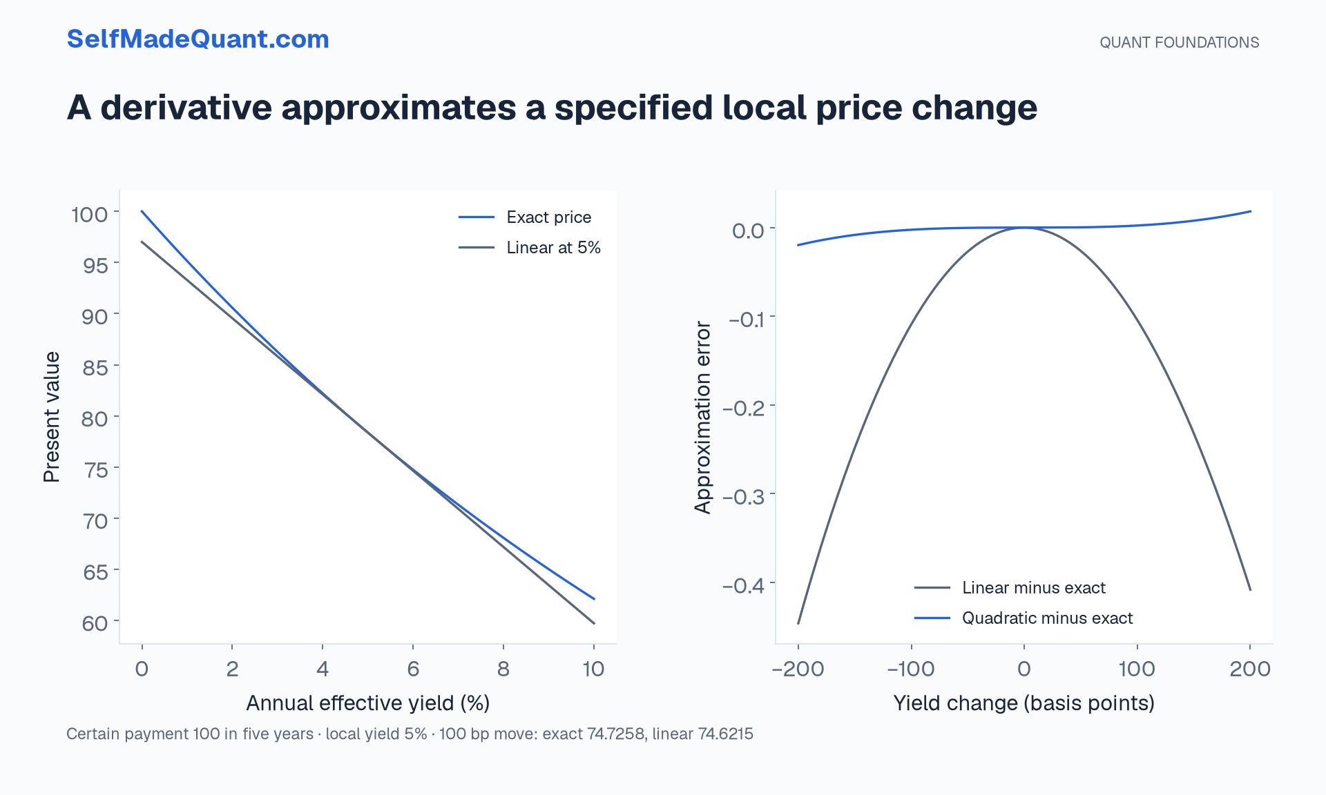
This is a certain-payment, flat-rate calculation. It contains no default uncertainty, optionality or changing term structure. A derivative with respect to a parallel yield input is not automatically a hedge against every movement in a real yield curve.
Partial derivatives say what stays fixed
Real models often have several inputs: a spot price, multiple rates, volatility parameters and time. A partial derivative changes one coordinate while holding the others fixed. That qualification is part of the mathematical definition and part of the economic interpretation.
If volatility changes with spot in your market model, the total response along that relationship can differ from the partial derivative holding volatility fixed. Neither calculation is universally the correct hedge. They answer different questions about which inputs can move together.
The chain rule describes the chosen relationship. Before applying it, say whether you are changing an independent model input, following a fitted surface or considering a specified scenario. A sensitivity calculated from a model inherits that model's assumptions.
Use finite differences as a check
def price(y):
    return 100 / (1 + y) ** 5

y = 0.05
h = 0.00001
central = (price(y + h) - price(y - h)) / (2 * h)
analytic = -500 / (1 + y) ** 6
print(round(central, 3), round(analytic, 3))
# -373.108 -373.108
A central difference evaluates the model on both sides of the starting input. For a smooth function it can be a useful independent implementation check. An extremely small step does not guarantee a better answer: subtracting nearly equal floating-point prices can magnify rounding effects.
Compare several reasonable step sizes. Look for a region of stable answers rather than one number that happens to agree. Keep rate conventions consistent across the analytic function and the numerical perturbation.
What to learn next
Build comfort with derivatives, partial derivatives, Taylor expansions, gradients and constrained optimisation. Connect each technique to a calculation you can explain in words. Integration then extends the toolkit to accumulated quantities and expectations over continuous distributions.
For each sensitivity, record the baseline, shocked variable, perturbation size, held-fixed inputs and exact repricing check. This short record prevents a plausible Greek from becoming a misleading economic statement.
Until then, peace.
Go deeper with lessons, derivations and worked exercises behind this article.