Programming for quants: a timestamp is part of the data

Published 13 October 20263 min readMaths / Finance / Programming for quants:Part 1 Part 2 Part 3 Part 4Part 5Part 6

A fast table join can build a backtest that knows the future. A missing label can attach the right return to the wrong asset. Quant programming starts with preserving the meaning of data through each transformation.

You need more than Python syntax. You need to know what each row represents, which keys identify it, which units its values use and when the information became available. Those decisions connect the program to the experiment it claims to implement.

We will use a small event-timing example, then connect it to labelled arrays and missing values. The goal is a pipeline you can inspect before you optimise its speed.

Observation time and availability time can differ

Suppose a hypothetical indicator describes conditions at 09:00 but is first available at 09:05. You make a decision at 09:02. The indicator's observation timestamp precedes the decision, but its value is still unavailable.

Joining by observation time would give the decision information it could not have received. A causal join needs the publication or availability timestamp appropriate to the intended use.

For a decision at 09:07, the 09:05 release may be eligible. If a revised value arrives at 10:00, it must not replace the originally available value in an earlier decision unless the experiment explicitly studies that revision.

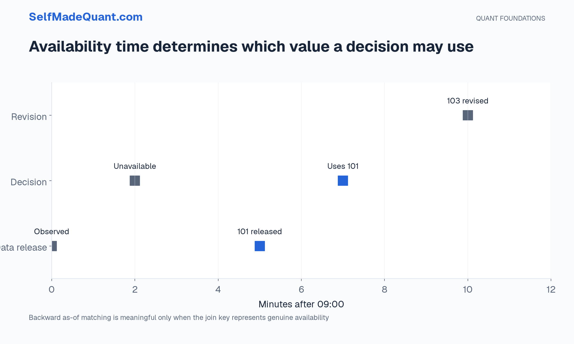
A timeline separates observation, publication and decision times; labelled data prevent accidental array alignment

This is a teaching timeline. Real datasets can have vendor delays, exchange timestamps, receipt timestamps and revisions. A single field called date rarely captures all of those meanings.

Match the latest eligible observation

An as-of join can select the latest record at or before a decision time. In pandas, backward merge_asof supports this matching direction on appropriately sorted inputs. Grouping and tolerance parameters help specify which series can match and how stale a record may be.

Those options implement a matching rule. They do not tell you whether the chosen timestamp represents real availability. A backward join on the wrong clock can still leak future information.

For a tiny example, the rule can be written without any library:

releases = [(5, 101.0), (10, 103.0)]  # minutes after 09:00
def available_value(decision_minute):
    eligible = [(t, value) for t, value in releases
                if t <= decision_minute]
    return max(eligible)[1] if eligible else None

print(available_value(2), available_value(7))
# None 101.0

Here release times are unique and values are already versioned as releases. With duplicate times, multiple instruments or revisions, define the tie-break and grouping rules explicitly. An implicit ordering can make results depend on the input file's row order.

Labels are a modelling safeguard

An array operation knows positions, not economic identities. If your weight vector is ordered A, B and your return vector is ordered B, A, a dot product will run and answer the wrong question.

Validate keys before converting labelled tables into arrays. Check uniqueness at the intended grain, sort deliberately and retain the mapping between each array column and its asset. Reject an unexpected duplicate rather than silently aggregating it through a convenient join.

Shape checks are necessary but insufficient. Two arrays can have identical shapes and incompatible labels, currencies or horizons. A helpful schema describes both computational structure and economic meaning.

Missing does not mean zero

A missing return might mean the instrument did not trade, a vendor failed, the listing ended or your query omitted a row. Replacing all missing returns with zero makes a strong economic assumption about every one of those cases.

Forward-filling a price also changes the implied return process. It can be appropriate for a carefully specified valuation convention, but it should not quietly become evidence that you could trade at an old quote.

Record the missing-data policy and test its effect. Distinguish a stale observation from a fresh zero change. Keep an explicit age or availability field when downstream decisions depend on that distinction.

Test what could have changed the conclusion

Change data strictly after a historical decision and recompute the earlier signal. A causal implementation should leave that earlier signal unchanged. This prefix check is useful for detecting accidental full-sample normalisation, centred windows or future joins.

Passing it does not establish that the dataset was point-in-time correct. A revised historical series can already contain hindsight in its earlier rows. Implementation causality and data provenance require separate checks.

After the model and data semantics are clear, learn vectorisation, SQL, profiling and packaging. Optimise measured bottlenecks while retaining a small, readable reference implementation for comparison.

The foundation resources contain runnable timing checks. Continue with tabular and time-indexed data. Consult the official pandas merge_asof documentation for supported matching options; the timing rules above define the economic experiment those options must implement.

Until then, peace.