Linear algebra for quants: turn positions into exposures

Published 13 October 20263 min readMaths / Finance / Programming for quants:Part 1Part 2 Part 3 Part 4 Part 5 Part 6

A portfolio can contain twenty securities and still make one concentrated economic bet. Counting names does not tell you how their risks combine. Linear algebra gives you a way to describe the positions, map them into exposures and check the calculation without losing track of units.

Start with two assets rather than a large covariance matrix. Suppose their returns over one common horizon are r1 and r2. Put 60% of capital in the first and 40% in the second. With weights fixed at the start of that horizon, portfolio return is 0.6r1 + 0.4r2, before costs and intermediate cash flows.

The vector notation packages that accounting identity. It does not supply a forecast or make the weights optimal. Understanding that distinction is a useful starting point for learning quant mathematics.

A vector needs an order and a unit

Write the weights as a column vector w and returns as a column vector r, using the same asset order. Their dot product gives portfolio return.

r_p=w^{\top}r=\sum_{i=1}^{n}w_i r_i.

Weights are dimensionless fractions of beginning capital; returns are dimensionless changes over the stated period. Dollar profit equals beginning capital multiplied by this portfolio return, under the assumptions above.

If asset returns are 2% and −1%, the portfolio return is 0.8%. An account beginning at 100,000 has a gross gain of 800. Entering the numbers as 2 and −1 instead of 0.02 and −0.01 produces a hundredfold error while leaving every matrix dimension valid.

Names matter too. Multiplying a weight array ordered A, B by returns ordered B, A computes a different portfolio. A successful numerical operation does not establish correct economic alignment.

Matrices map positions into another description

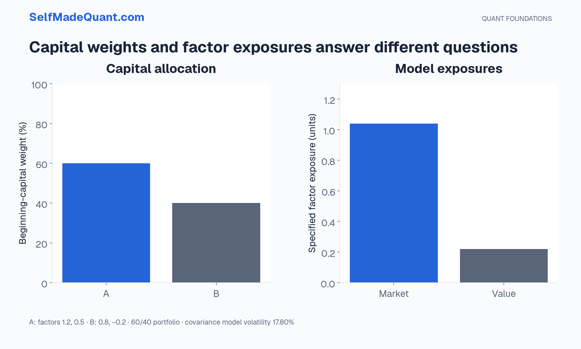
Suppose a two-row matrix records each asset's exposure to a market factor and a second illustrative factor. Asset A has exposures 1.2 and 0.5; B has 0.8 and −0.2. With assets as columns, multiplying the matrix by w gives exposures 1.04 and 0.22.

These are weighted combinations of the supplied asset exposures. They are not probabilities. A negative factor exposure is allowed even when both security weights are positive.

Check the shape before calculating: a two-factor-by-two-asset matrix times a two-asset vector returns a two-factor vector. In a larger system, the dimensions should express the same economic mapping. Writing down those dimensions can catch a transposition error earlier than inspecting its output.

Portfolio weights map to returns and factor exposures; labels retain their economic units

The same idea appears in scenario analysis. Give each row a scenario and each column an asset's scenario return. Multiplying by the portfolio weights produces one return per scenario. A scenario matrix describes specified shocks; it is not automatically a statistical model of how often they occur.

Covariance keeps the joint behaviour

Suppose the assets have annual volatilities 20% and 30%, with correlation 0.1. The covariance is 0.1 × 0.2 × 0.3 = 0.006. All inputs refer to the same horizon and return convention.

For the 60/40 weights, variance is 0.6² × 0.04 + 0.4² × 0.09 + 2 × 0.6 × 0.4 × 0.006 = 0.03168. Volatility is the square root, approximately 17.80%.

Adding the two weighted volatilities instead gives 24%. That is the perfect-positive-correlation case, not the answer for correlation 0.1. Dependence determines how much diversification the model permits.

The matrix expression is w-transpose times Sigma times w. A valid covariance matrix is positive semidefinite: it cannot assign negative variance to a linear combination. Positive semidefinite does not guarantee invertibility. Two duplicated return series can make the matrix singular without making it an invalid covariance matrix.

A small calculation you can audit

weights = [0.6, 0.4]
returns = [0.02, -0.01]
covariance = [[0.04, 0.006], [0.006, 0.09]]
portfolio_return = sum(w * r for w, r in zip(weights, returns))
variance = sum(weights[i] * covariance[i][j] * weights[j]
               for i in range(2) for j in range(2))
print(round(portfolio_return, 4), round(variance ** 0.5, 6))
# 0.008 0.177989

The runnable foundation lab repeats this calculation and checks the labelled exposure mapping. There is no random input in this example. If you later simulate returns, specify the generator and seed as well as the covariance model.

Learn dot products, matrix multiplication, transposes, linear systems and eigenvalues through questions like these. What is the input? What is the output? What unit does each component carry? Which economic relationship does the operation encode?

The foundation resources contain the code and visual notes. Continue with vectors and matrices or expectation, variance and covariance.

For the underlying matrix theory, see MIT's positive definite matrices and minima. The portfolio numbers here are independent illustrative calculations, not estimates from market data.

Until then, peace.