Trading costs and slippage: when a profitable backtest stops working
A trading rule earns 1.13% on our synthetic sample before costs. Charge 5 basis points on each traded dollar, and its account loses 7.49%.
The rule, prices and signal timestamps are unchanged. The economic calculation is different because trading consumes cash and reduces the capital available for later positions.
This article separates the costs, shows where they belong in the ledger, and explains why subtracting one guessed percentage from the final return is not the same experiment.
Start with a traded dollar
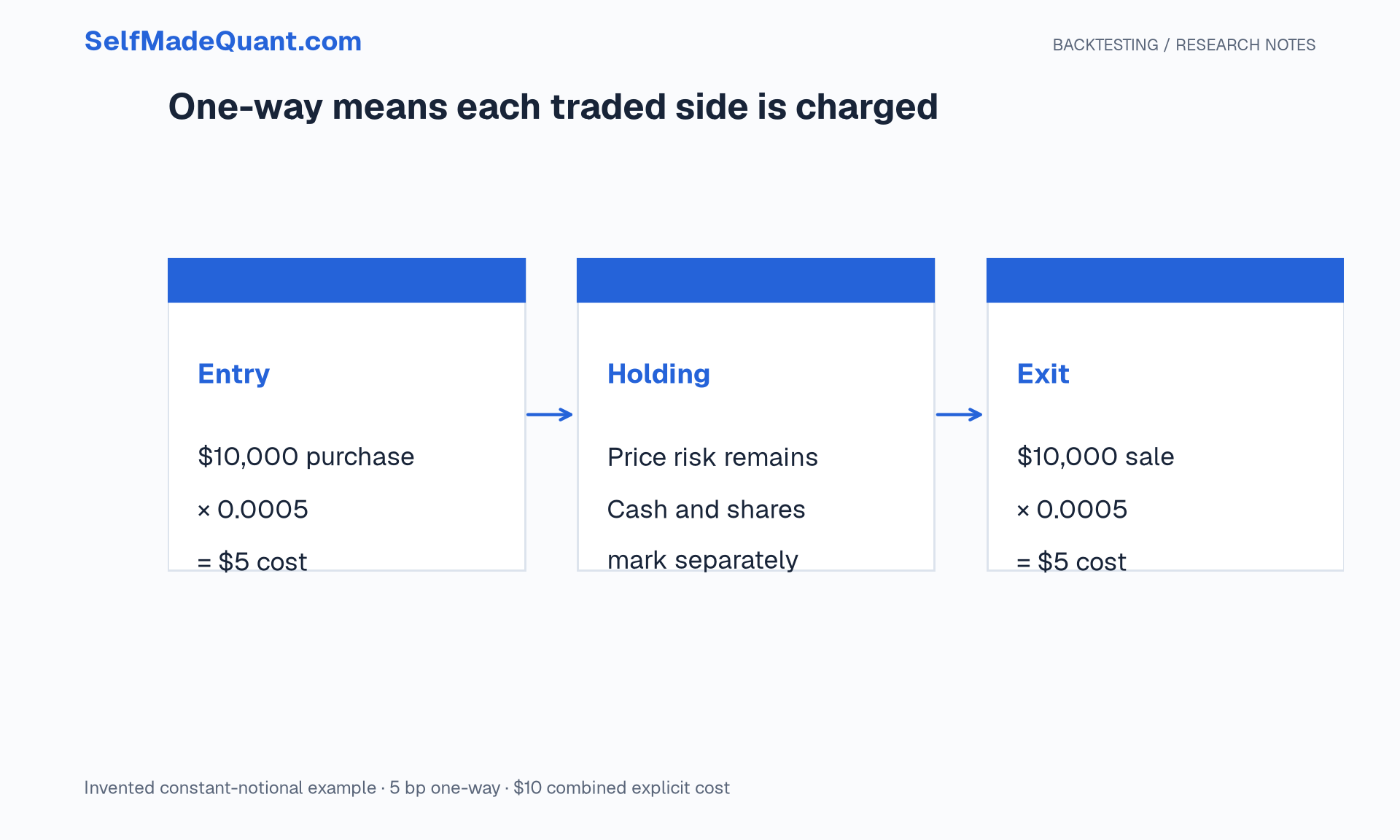
One basis point is 0.01%, or 0.0001 as a decimal. A 5 bp charge on 5. Buying and later selling approximately 10 of costs.
Write “one-way” or “round-trip” beside every quoted rate. Confusing them can double or halve the intended charge.
For an order whose absolute traded notional is N, a simple proportional model is:
This is the model used in our teaching ledger. The 5 bp rate is an assumption, rather than an estimate from observed fills.
Four quantities often mixed together
These quantities overlap depending on definitions. If an implementation-shortfall estimate already measures the fill against the decision midpoint, adding a separate spread penalty may double-count part of the same execution loss.
Our scalar cost rate bundles execution friction into a deliberately simple penalty. It does not identify commissions, spread, delay and impact individually.
The cash account makes the timing visible
On entry, the strategy spends money on shares and on the entry charge. It therefore buys fewer shares than the frictionless strategy. On exit, the sale produces cash less the exit charge.
Those differences affect subsequent position sizes. Compare two accounts running the same binary signal sequence: the one with higher costs generally brings less capital to future entries in this model.
That is why our final wealth difference is not equal to the sum of the cost account from only one run. Removing costs also changes later holdings and their gains or losses.
In the baseline synthetic run, explicit costs sum to 8,611.28. The remaining difference comes from the different capital paths and resulting position sizes.
Both figures are useful. The first answers how many dollars the baseline account paid in explicit charges. The second compares two complete capital trajectories.
Count turnover with a convention
Buying approximately a full account and eventually selling it contributes approximately two units. Market gaps and the cost budget mean those units need not equal exactly two.
For the fixed 20-session rule, cumulative one-way turnover is approximately 177.88 over 1,432 evaluated sessions. Its mean daily turnover is approximately 0.1242. Multiplying by 252 gives roughly 31.30 units per assumed year.
This is different from a convention that divides traded notional by two, and different from counting completed trades. A strategy can have few trades and large notional changes, or many tiny trades.
State the definition before comparing reports.
A first-order break-even calculation
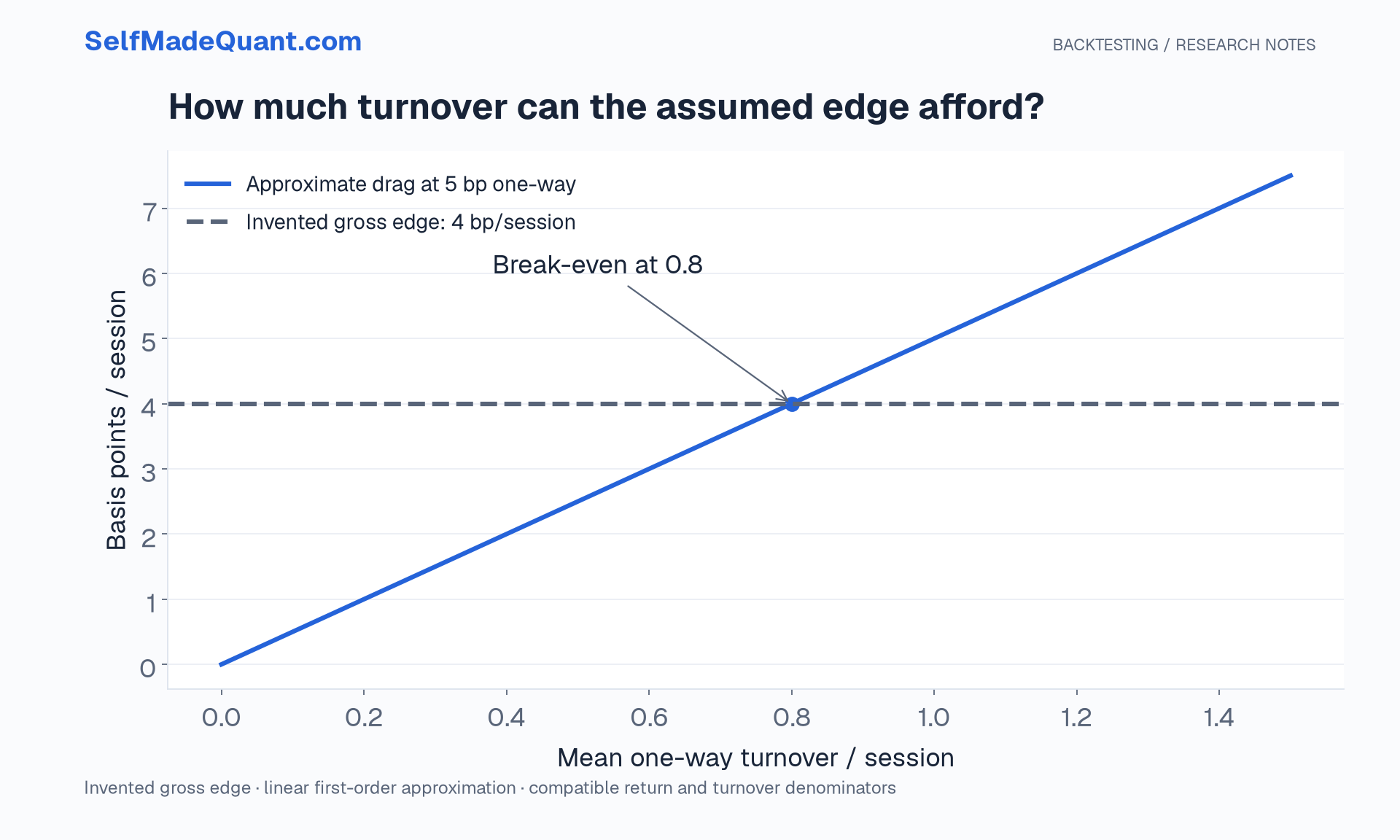
Suppose a strategy earns an expected gross return of 4 bp per session and turns over 0.8 times wealth per session under a compatible denominator. At a 5 bp one-way cost, its approximate cost drag is 0.8 × 5 = 4 bp per session.
The gross estimate has already been consumed. This rough comparison ignores compounding, state-dependent sizes and nonlinear impact, but it is enough to question a fragile result.
For compatible average gross return g and turnover τ, the first-order break-even one-way rate is:
A positive mean is still an estimate with uncertainty. It does not become reliable merely because we can divide it by turnover.
Stress the fixed policy
Run the same 20-session signal rule with several rates. Do not re-optimise the rule at each rate and call that a pure cost sensitivity test.
| One-way cost | Terminal wealth | Total return |
|---|---|---|
| 0 bp | $101,125.45 | +1.13% |
| 5 bp | $92,514.17 | −7.49% |
| 10 bp | $84,636.17 | −15.36% |
| 25 bp | $64,803.58 | −35.20% |
| 50 bp | $41,527.44 | −58.47% |
All rows use the same seeded synthetic fixture, $100,000 initial cash and sessions 80–1511. Entry and exit charges are applied to actual notional, including final liquidation.
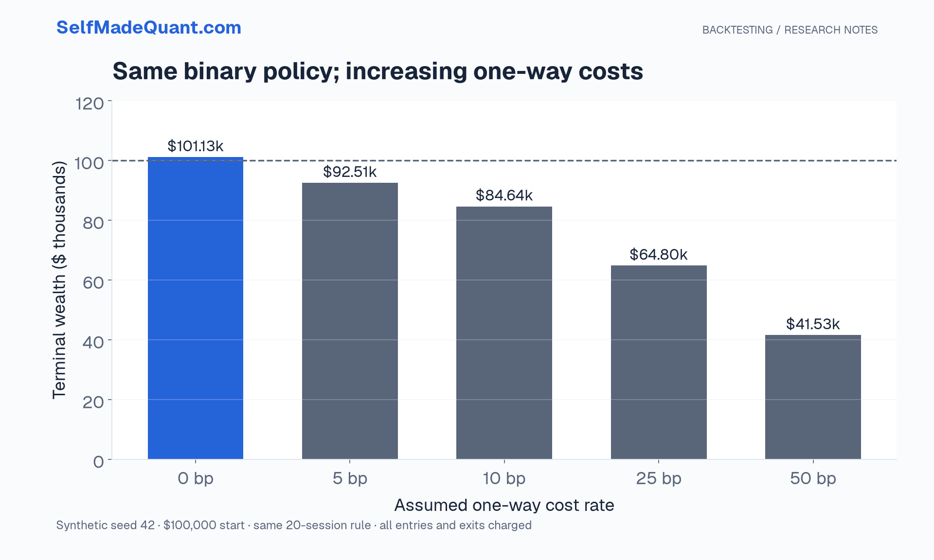
The table establishes sensitivity under this model. It does not establish which rate is realistic for a particular market. To estimate that, collect relevant execution data and compare orders of similar size, urgency and market conditions.
Why “the close touched my limit” is insufficient
A limit order can be displayed without filling. Earlier orders may have priority. The traded quantity may be too small to reach your place in the queue. A daily high or low also does not tell you the sequence of events inside the bar.
For the same reason, daily bars can fail to tell you whether a stop or profit target happened first. Resolving an ambiguous sequence in your strategy's favour introduces another optimistic assumption.
Our lab avoids those order types. It models next-open execution and a known terminal-close sale. Those remain price proxies, with costs supplied by assumption.
Add costs to the research question
An economic hypothesis should explain why a signal might predict a move large enough to compensate for obtaining and managing the position. It should also explain why the opportunity is not exhausted by the costs of acting on it.
A slower rule may trade less, but it can react later and hold unwanted exposure longer. Lower turnover alone is not a complete optimisation objective.
Before changing the rule, write the proposed cost mechanism, its units, and the observations that would support it. Keep the original sensitivity run as a reference.
Until then, peace.
Go deeper with lessons, derivations and worked exercises behind this article.