Sharpe ratio, drawdown and turnover: how to evaluate a trading strategy

Published 13 October 20265 min readBacktesting and strategy evaluation:Part 1 Part 2 Part 3 Part 4Part 5

Two strategies finish with the same profit. One holds through a 40% decline. The other trades every few minutes and depends on fills that disappear when you add a modest execution penalty.

Their final returns do not describe the same experience or the same economic exposure.

A useful strategy report connects the return to the capital path, risk, activity and assumptions that produced it. We will construct that report from our executed backtesting lab, keeping full-period description separate from the later validation segments.

Begin with the account return

Our account has no external deposits or withdrawals. Its session return is closing wealth divided by previous closing wealth, minus one. Initial wealth supplies the denominator for the first evaluated session.

The cumulative return compounds those account returns:

R=\prod_{t=1}^{T}(1+r_t)-1.

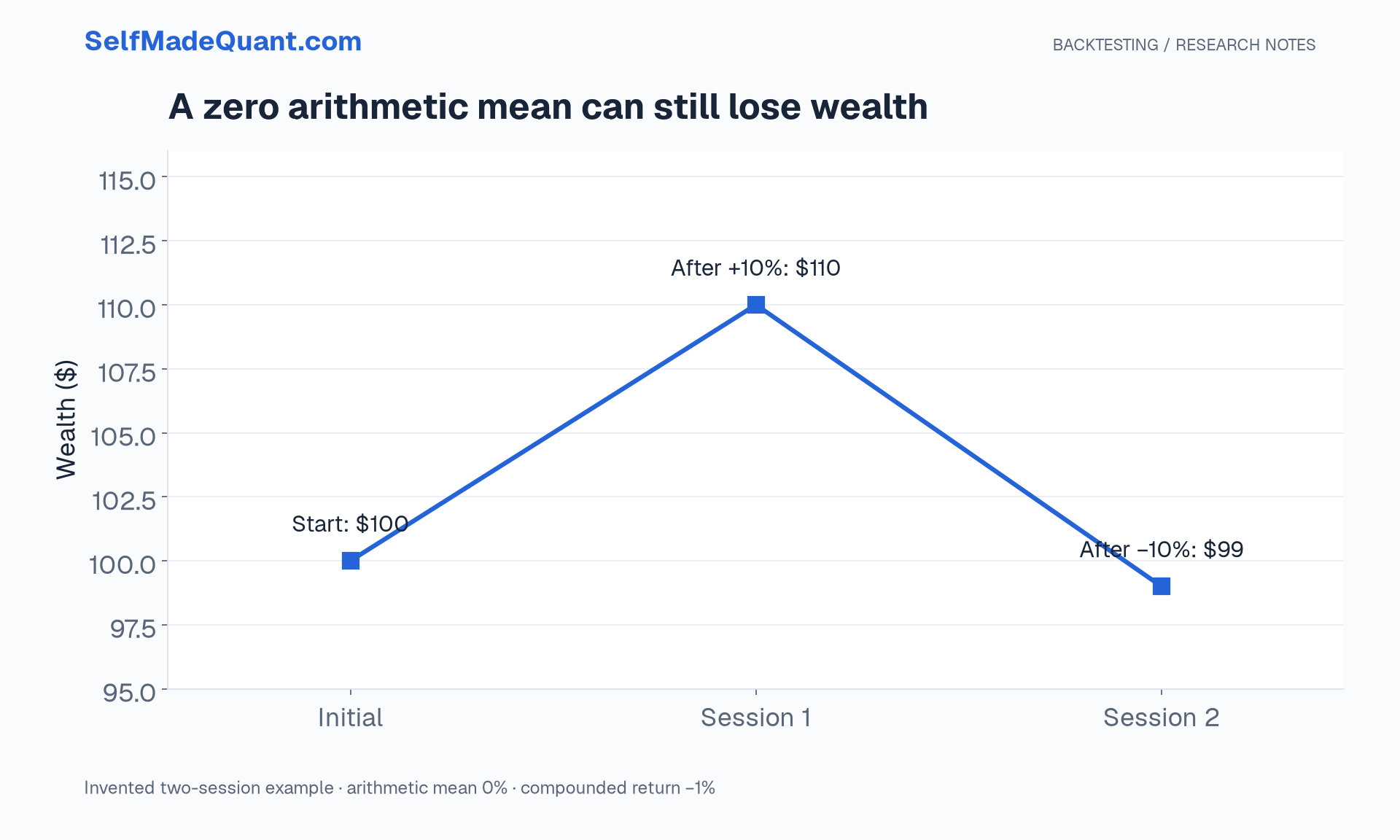
Adding returns is an approximation. A gain of 10% followed by a loss of 10% leaves $99 from$ 100, a 1% loss. The arithmetic mean of the two returns is zero.

For an assumed 252 sessions per year, the annual compound growth rate is:

\mathrm{CAGR}=\left(\frac{W_T}{W_0}\right)^{252/T}-1.

Our numbered synthetic sessions are not a real exchange calendar. The 252 convention translates the observation count into an illustrative annual scale. A real account also needs a policy for dates, missing sessions and external cash flows.

Compounding distinguishes account growth from arithmetic average return

Invented two-session example: $100 becomes$ 110, then $99.

State what the Sharpe ratio measures

The sample Sharpe ratio divides average excess return by its sample standard deviation. For our zero-interest teaching account, excess return equals account return.

The conventional annualised calculation is:

\widehat{S}_{\mathrm{annual}}=\sqrt{252}\,\frac{\overline{r}}{s_r}.

Use the sample standard deviation with denominator T−1, and include the account's cash sessions. Dropping flat sessions changes the question into performance conditional on activity.

The square-root scaling relies on assumptions about how returns aggregate. Serial dependence can make that conventional conversion misleading. Andrew Lo's The Statistics of Sharpe Ratios develops the estimation and time-aggregation issues. Our output labels this statistic sharpe_iid to make its conventional scaling visible; that label does not prove the strategy returns are independent.

Even when underlying synthetic increments are independent, a strategy's changing exposure, costs and decision process deserve separate examination. An estimated ratio also has uncertainty, especially after selecting a winner from many candidates.

A loss can coexist with a positive arithmetic Sharpe

Buy and hold in our full-period fixture loses about 8.39% after costs but has a conventional sample Sharpe slightly above zero, approximately 0.015.

This is not an accounting contradiction. The statistic uses an arithmetic mean of session returns. Terminal growth uses their product. Volatility can create a gap between arithmetic average and compound growth.

A report that displays only Sharpe can therefore hide an account that lost money. A report that displays only total return can hide severe variability. Show both and explain the inputs.

For the fixed 20-session strategy with 5 bp costs, total return is −7.49% and the conventional Sharpe is approximately −0.036. Its conventional annual volatility is approximately 13.36%.

Specify the Sortino denominator

Sortino-style ratios replace total return variability with a downside measure relative to a chosen target. Conventions differ, so write the one you use.

Our target is zero per session. Define downside deviation by averaging squared negative returns over all T sessions:

d=\sqrt{\frac{1}{T}\sum_{t=1}^{T}\min(r_t,0)^2}.

We report the mean return divided by d and multiply by the same conventional square-root factor. This is different from taking the standard deviation of negative observations alone. If there are no downside observations, the denominator is zero; report the statistic as undefined rather than quietly replacing it with a large number.

A threshold other than zero changes both the interpretation and calculation. Do not compare numbers from incompatible definitions.

Measure the decline from an actual peak

Let H be the highest account wealth observed so far, including initial capital. Drawdown is:

D_t=\frac{W_t}{H_t}-1.

Maximum drawdown is the most negative observed value. It is a path statistic from this sample, rather than a guaranteed bound on future losses.

A 20% decline from $100 leaves$ 80. Recovering to $100 requires a 25% gain. A 50% decline requires a 100% recovery. Loss and recovery percentages use different starting amounts.

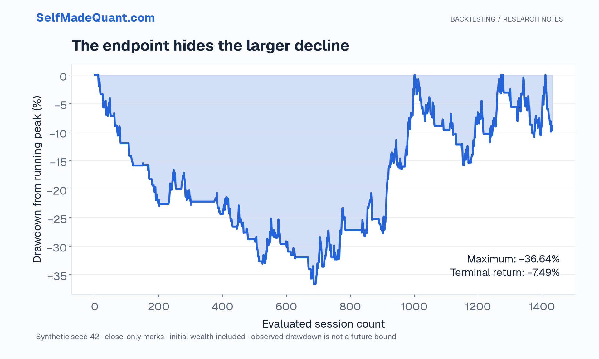
Drawdown is measured against the running wealth peak, including initial capital

Synthetic fixed-window strategy after 5 bp one-way costs. Maximum drawdown is approximately 36.64%.

Our fixed strategy's −7.49% terminal return coexists with a roughly 36.64% maximum drawdown. Much of the decline was recovered before the final observation. The endpoint alone hides that experience.

Intraday drawdowns can also exceed a close-only calculation. The lab marks at closes and cannot claim to measure every loss within a session.

Put turnover and exposure beside risk

The fixed strategy's mean binary signal exposure is approximately 49.30%. That reports the fraction of evaluated sessions with an invested target. It is not an intraday time-weighted exposure measure, and the final session's target can be one even though the scheduled closing liquidation leaves zero terminal shares.

Cumulative one-way turnover is approximately 177.88. The convention is absolute traded notional divided by previous closing wealth, summed over sessions. Explicit costs sum to $7,292.03.

Those quantities help explain why the net and gross results differ. They also show why a lower-volatility strategy may simply have spent more time in cash.

Do not treat cash exposure as a flaw. Treat it as information needed to compare strategies on compatible terms.

Compare like with like

Full-period descriptive run	20-session strategy	Buy and hold
Evaluated sessions	1,432	1,432
Total return, after 5 bp costs	−7.49%	−8.39%
Conventional annual volatility	13.36%	19.10%
Conventional annual Sharpe	−0.036	0.015
Maximum closing drawdown	−36.64%	−51.03%
Mean invested signal	49.30%	100.00%

These rows match sample boundaries and cost conventions. They do not make the exposures identical. A cash-and-market comparison can contextualise risk reduction, but claiming forecasting skill needs further evidence.

A strategy report includes return, risk, activity and evaluation boundaries

Full-period description, walk-forward evaluation and frozen final evaluation are separate experiments with different session ranges.

Keep the validation result in its own table

The walk-forward article evaluates a selection procedure across 676 later sessions. Its net total return is 40.33%. The separate frozen final run covers 252 sessions and earns 8.15%, with a conventional Sharpe of about 0.62 and maximum closing drawdown of about 9.26%.

Do not place those returns beside the full-period baseline without their dates or session ranges. Different periods can dominate the apparent ranking. The final account also starts separately with $100,000; its wealth is not an extension of the earlier$ 140,331.25 account.

A positive selected result on a synthetic random path illustrates sampling variation. It does not turn this lab into evidence of a profitable market strategy.

Finish with an inspectable research record

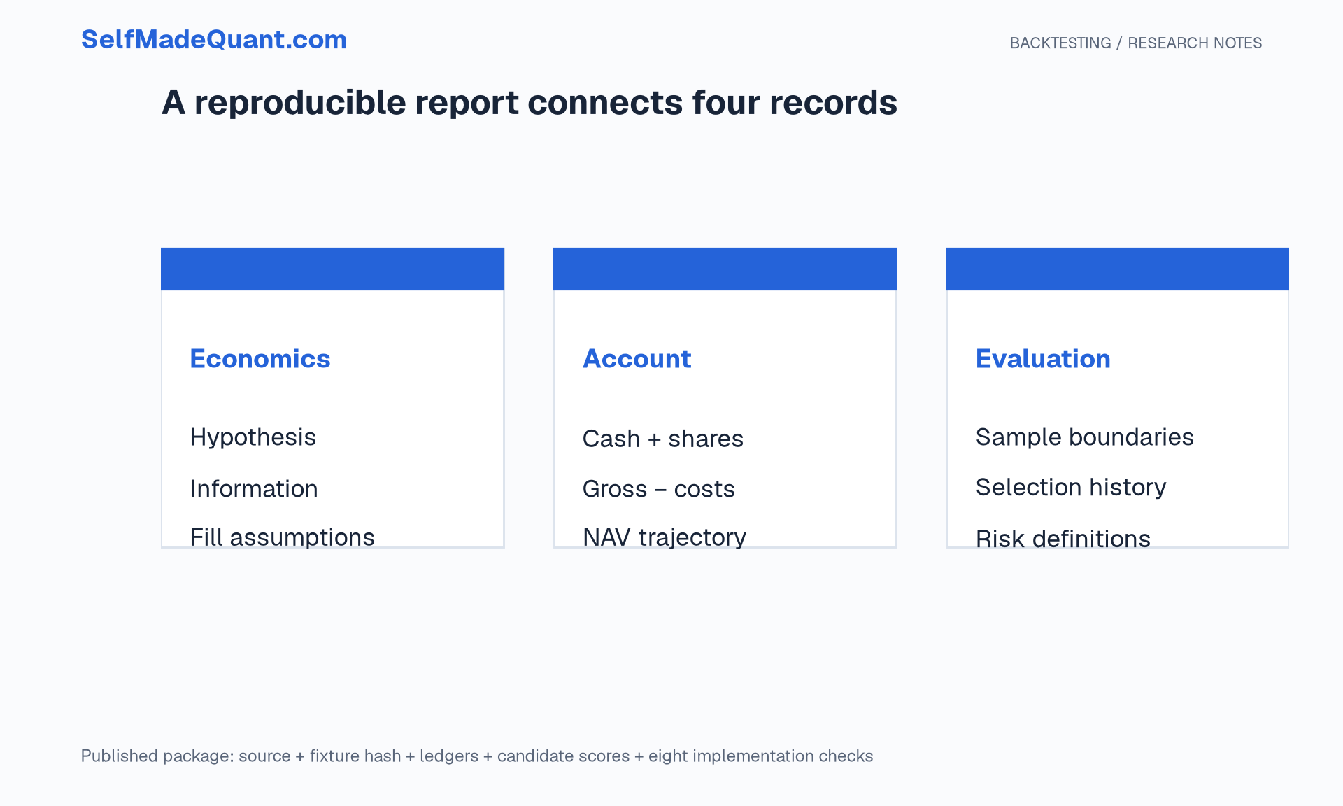
The reader package contains source code, exact fixture, a SHA-256 fixture hash, cash ledgers, candidate scores, sample boundaries and eight checks. Those checks cover accounting reconciliation, affordable positions, causal trailing signals, terminal liquidation, fixed-policy cost sensitivity, non-overlapping evaluation blocks, final-segment separation and a hand-calculated cash example.

Passing them supports the implementation claims they test. It does not validate a real-data source, execution venue or economic hypothesis.

When reviewing another backtest, request one representative trade, one cash reconciliation, the cost convention, the comparison period and the research-selection history. Then ask what the strategy was allowed to know at each decision.

That sequence gives you a much better starting point than asking whether the equity line is smooth.

Download the complete backtesting lab and visual notes, practise quantitative reasoning in the interview tools, or explore the learning programmes. You can subscribe separately on Substack for the next series.

Until then, peace.