Walk-forward validation in Python: test the rule that chooses the strategy

Published 13 October 20265 min readBacktesting and strategy evaluation:Part 1 Part 2 Part 3Part 4Part 5

You test five moving-average windows. One gives the best Sharpe ratio. You select it and present the same period as evidence that the selected strategy works.

The period helped choose the winner. Its winning score describes that selection exercise.

Walk-forward validation repeatedly chooses or fits a rule using earlier observations, then evaluates the resulting choice over a later block. The object being evaluated is the complete procedure, including how parameters are selected, when they are updated and how positions change.

We will implement that procedure explicitly. Then we will preserve a final segment for a frozen evaluation.

Declare the candidate set

Our candidates use trailing means of 5, 10, 20, 40 or 80 closes. Each uses the same binary rule and the same next-open execution convention from the first article.

Choose the candidate with the highest conventional annualised sample Sharpe ratio on the permitted training block, after a 5 bp one-way cost. Break ties by selecting the smaller window.

Those decisions are part of the algorithm. So are the 504-session trailing training length and the nominal 126-session evaluation length. Trying many alternatives for those choices is additional research, even if only five candidate windows appear in the final table.

Our synthetic fixture was generated with seed 42 before inspecting strategy outcomes. Its overnight and intraday returns are independent draws with constant parameters. A positive evaluation result can occur by chance; the generator contains no designed predictive moving-average signal.

Put the boundary on a numbered session

Number sessions from zero through 1511. Reserve sessions 1260–1511 as the final 252-session segment.

Use the first 80 sessions as available historical context for the initial training evaluation. The first training return block is sessions 80–583, giving 504 sessions. Historical observations before session 80 can initialise indicators without contributing training returns.

At the end of session 583, select a window. Execute the first evaluation decision at session 584's open. That signal may use the completed close at 583; it cannot use the opening or closing price at 584 to decide the window.

Evaluate through session 709. Then move the training window forward and repeat. There are five full 126-session evaluation blocks and a final 46-session block ending at 1259, giving 676 evaluation sessions in total.

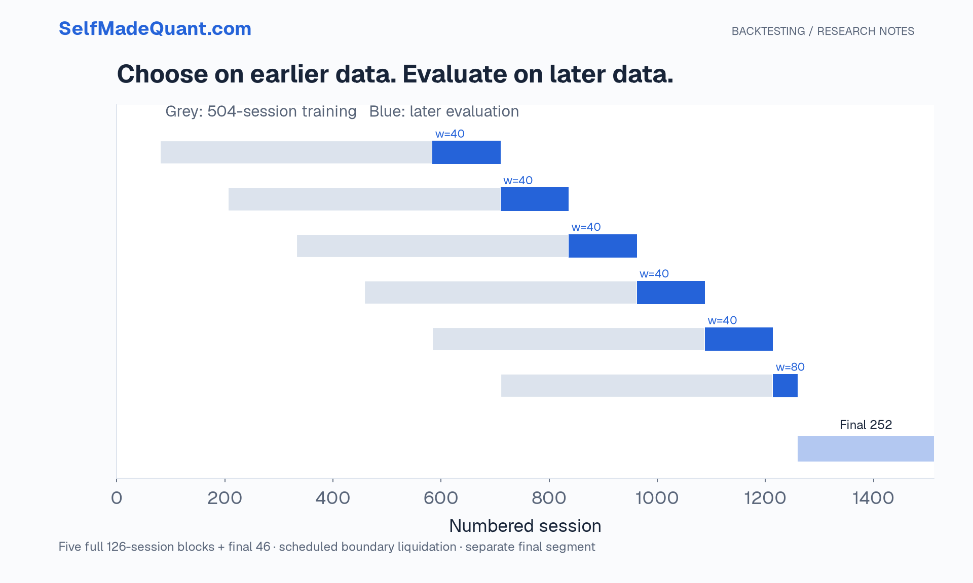
Earlier observations select a window; subsequent blocks evaluate it; the last 252 sessions remain separate

Session indices are inclusive in labels. The final short block keeps every evaluation observation before the reserved segment.

The training windows overlap. The evaluation blocks do not. Later training windows are allowed to use observations that were earlier evaluation data, because those observations would then be in the past. That is a declared update rule, rather than retroactively changing an earlier decision.

Separate warm-up from fitting

A trailing mean needs historical context. At an evaluation boundary, retain completed closes from the training history so that the chosen indicator is ready for the next open.

This does not require carrying the previous training simulation's portfolio into the evaluation. Our protocol starts each evaluation block in cash and liquidates at its scheduled final close, paying costs. The next block starts with the resulting capital.

That forced liquidation is a modelling choice with an economic cost. Another procedure might carry positions across updates and reconcile them with a newly selected rule. It should simulate those trades explicitly.

Do not concatenate independently funded blocks and assume the resulting equity line is one continuous account. We pass the previous block's ending cash into the next simulation, so capital compounds across the sequence.

Select without reading the evaluation outcome

The package's selection function accepts the training start and its exclusive end. It scores candidates using only that return block. Indicators have access to earlier completed prices for warm-up.

import pandas as pd
from backtest import select, simulate, metrics

data = pd.read_csv('synthetic-prices.csv')
window, scores = select(data, start=80, end=584)
evaluation = simulate(data, window=window, start=584, end=710)
print(len(evaluation))
# 126

The code's full dataset is present in memory, but the signal dependency and scoring slices are constrained. Our separate prefix-invariance check verifies the trailing signal before a cutoff is unchanged when later observations are removed. A stronger production interface can pass only permitted prefixes to selection routines.

Record the chosen window and all five training scores at every boundary. That record makes it possible to check whether the published selection really followed the stated rule.

What the executed experiment produced

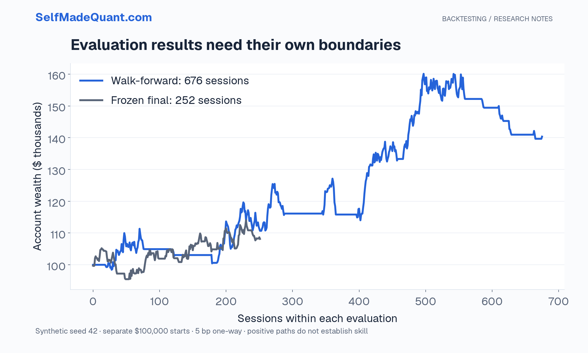
The chained walk-forward evaluation turns $100,000 into$ 140,331.25 over its 676 sessions, after the assumed costs. Its total return is 40.33%, and its conventional sample Sharpe is approximately 0.96 under 252-session square-root scaling.

This result is not comparable to the fixed 20-session strategy's full-period return without matching dates. The earlier article's fixed-policy table covers 1,432 sessions, including different observations. A shorter favourable evaluation interval can improve a chart even when the algorithm has no predictive advantage.

The lab publishes both ledgers so readers can align periods. The synthetic data-generating process is also known. That context is stronger evidence about the absence of designed predictability than a pleasing single path is evidence of discovered skill.

Net wealth across the walk-forward evaluation and the separately funded final segment

Both panels start with $100,000 for readability. The final segment is a separate frozen run, not the continuation of the walk-forward capital.

Freeze the last decision

At the end of session 1259, use the preceding 504-session training block, sessions 756–1259, to select one window. The executed selection chooses five sessions.

Freeze that choice through sessions 1260–1511. The final run starts with a separate $100,000 and ends with$ 108,147.71 after costs, an 8.15% gain. Its maximum drawdown is approximately 9.26%.

Once that outcome has been inspected, the segment has been consumed for this research exercise. If you change the candidate set or training rule in response, a fresh claim of independent evaluation needs new observations or a clearly labelled different research design.

“Untouched” is a property of the research history, not a permanent label attached to dates.

Why a random split is a different question

Randomly allocating rows can train on observations from later dates than the ones being evaluated. For a process intended to run forward in time, that does not reproduce its information schedule.

scikit-learn's TimeSeriesSplit documentation describes chronological splits and a gap parameter. A splitter supplies indices; you still need to handle preprocessing, publication times, labels, trading and parameter selection correctly.

If a label at date t uses the following ten sessions, some training labels near a boundary can include outcomes from the evaluation period. Remove the overlapping labels or design a suitable gap. A generic one-row gap does not automatically solve a ten-session dependency.

Our baseline's selection objective uses completed trading returns and a previous-close signal. It has no forward-ten-session prediction label. Do not add label purging mechanically without identifying the dependency it is meant to remove.

Validation is evidence about a specified process

The experiment demonstrates a reproducible selection and accounting workflow. It does not establish that five windows, 504 training sessions or a 126-session update schedule are universally appropriate.

Keep a research log of candidate sets, discarded variants and each evaluation you inspected. Bailey and coauthors' backtest-overfitting paper explains why selection history matters when interpreting the winning result.

In the final article, we will turn this experiment into a compact report: returns, exposure, drawdown, costs and the assumptions behind each statistic.

Get the runnable selection log and visual notes in the backtesting resources. Subscribe separately on Substack for future series.

Until then, peace.