Does machine learning beat a simple trading strategy? Compare forecasts, positions and costs
This series uses zero and training-mean return forecasts, ridge regression and a shallow regression tree. Their final results are intentionally disappointing. The synthetic relationship changes after model selection, and both ML models perform worse than the simple forecasts on final mean-squared error.
That result does not show that ML fails in every market. It shows why the evaluation should be capable of returning “no useful improvement” without changing the question until a preferred model wins.
Which simple baselines should financial ML beat?
For return forecasting, a zero forecast makes a clear claim: the experiment has not identified a conditional mean worth predicting. A training-mean forecast adds a constant estimated from eligible history. Neither requires a complex feature relationship.
For trading, include a no-trade baseline. It earns zero in the lab's unit-reference-capital P&L calculation and incurs no trading costs. A buy-and-hold or risk-matched benchmark can be useful for a different mandate, but it must represent the exposure and financing convention you intend to compare.
An appropriate simple rule may also be momentum, mean reversion or a volatility-based allocation. Specify it before looking at the final result. Selecting the best “simple baseline” from a large hidden search creates the same research-history problem as searching a large ML model family.
Our experiment compares all four forecasts on exactly the same 600 final return intervals. It excludes the impossible target-leakage control from the admissible ranking. All methods receive the same fixed position mapping and the same proportional cost model.
What does regularised linear regression add?
Ridge regression models expected return as an intercept plus a weighted sum of standardised features. Under this lab's convention it minimises:
The intercept is not penalised. The mean-squared-loss normalisation matters: an implementation that uses the sum of squared errors has a differently scaled penalty. Comparing two values called “alpha” requires checking their objective definitions.
Regularisation can reduce sensitivity to noisy correlated features, but it cannot guarantee stability after the underlying relationship changes sign. The lab selects alpha 0.1 from four declared candidates using chronological validation, then freezes the fitted model for the final block.
What does a regression tree add?
A tree partitions the feature space and predicts a training-sample mean within each leaf. It can represent threshold effects and interactions without requiring them to be written as a single linear equation.
That flexibility also makes sample size in each leaf important. Our transparent teaching implementation considers nine candidate quantile thresholds per feature at a node; it is a coarse tree, not a full production CART implementation. Validation chooses depth three with at least forty training observations per leaf.
Deepening the tree creates more local estimates. If those leaves contain little independent information, apparent structure can be noise. Financial observations sharing a regime or event make raw row counts an incomplete description of effective information.
Feature importance is not a causal explanation either. Correlated predictors can share or substitute for one another. Use held-out checks that preserve the timing structure, and interpret feature-attribution results within the model and data used.
What happens in the final sample?
The generator deliberately reverses the signal–return relationship at the final boundary. This is disclosed before interpreting the result. It is a designed stress test of generalisation, rather than evidence that an observed market had this particular break.
| Admissible forecast | Final MSE, decimal-return squared | Mean gross P&L, bp per interval | Mean net P&L at 5 bp per turnover unit |
|---|---|---|---|
| Zero | 0.00010490 | 0.000 | 0.000 |
| Training mean | 0.00010479 | 0.071 | 0.071 |
| Ridge | 0.00012473 | −7.056 | −7.661 |
| Shallow tree | 0.00012654 | −6.847 | −7.599 |
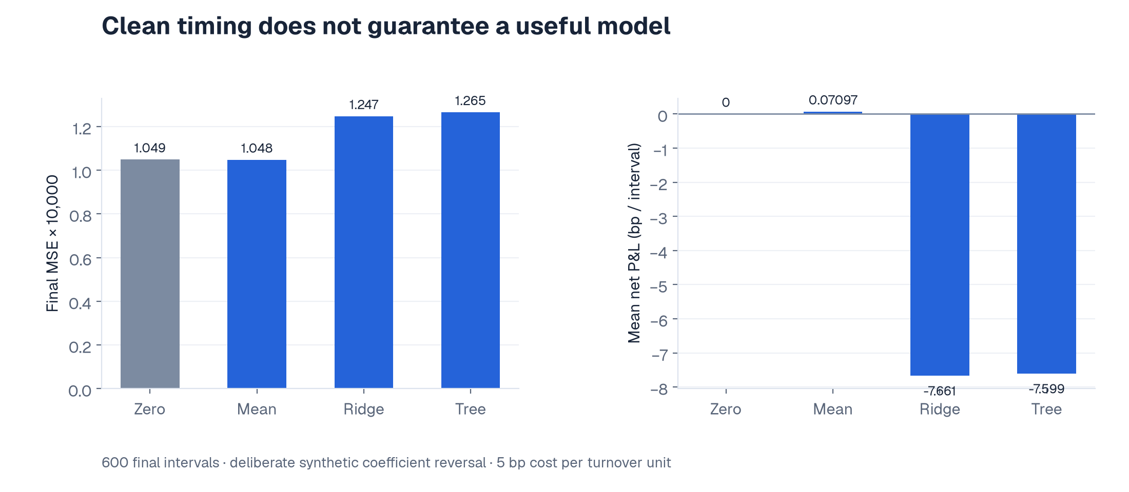
The training-mean forecast is close to zero. Its tiny positive final P&L on this path is not a demonstrated edge. Neither model family earns a strong claim from one synthetic seed, and the very small difference between the two losing ML strategies should not be promoted as a robust ranking.
Notice that the tree has worse MSE than ridge but slightly less-negative net P&L. The two metrics evaluate different objects. Forecast errors are squared uniformly; trading P&L also depends on prediction scale, realised return and turnover.
How should a forecast become a position?
The lab fixes the mapping before validation:
A predicted return of 0.5% maps to half a unit of exposure. The divisor is a stated scaling convention, not an optimised claim about Kelly sizing or risk targeting. Short exposure is permitted in the toy calculation; actual borrow availability and fees are omitted.
Positions earn the next synthetic open-to-open return. On a fixed reference capital, gross interval P&L is w_t times y_t. The model charges five basis points for each unit of absolute position change. It includes the initial entry and final liquidation as well as intermediate rebalances.
For positions +0.5 then −0.5, total turnover is 0.5 + 1.0 + 0.5 = 2.0 units. At five basis points per unit, total cost is ten basis points of reference capital. Calling five basis points a “round-trip cost” would describe a different assumption.
The cumulative output is an arithmetic sum of P&L on fixed reference capital. It is not a compounded buy-and-hold return series. The experiment does not enforce real margin, funding, liquidity or solvency rules.
Why can accuracy improve while trading gets worse?
Directional accuracy ignores the size of outcomes. A rule winning one basis point on 60% of trades and losing two basis points on 40% has expected P&L of −0.2 basis points before costs. A higher hit rate is not sufficient.
Regression MSE can also be dominated by observations that do not produce economically meaningful trades. Conversely, a threshold may reduce turnover while discarding some useful forecasts. Choosing that threshold using final P&L consumes the final sample just as selecting a model does.
If the real objective is a cost-aware allocation policy, design validation around that objective and its risk constraints from the start. The current lab deliberately selects by MSE and reports trading results separately, so their disagreement remains visible.
What evidence would support a stronger claim?
Use genuinely point-in-time market data, feasible execution and a declared research history. Compare relevant exposures and risk, not just raw cumulative profit. Examine different periods, cost assumptions, stability and uncertainty under dependence. A final result should survive the specific checks implied by the claim.
For this experiment, the honest conclusion is narrower: ridge and the coarse tree learn a relationship that does not survive the designed final reversal. Costs further reduce P&L. The no-trade baseline remains useful because the evaluation allows trading to be worse than doing nothing.
References
Until then, peace.
Go deeper with lessons, derivations and worked exercises behind this article.