Portfolio construction: define the portfolio before choosing an optimiser

A set of attractive forecasts does not tell you how much of each asset to own. You still need a budget, a risk description, a trading policy and a feasible set of positions. Portfolio construction connects those decisions to the account you can actually hold.

Start with two assets. Their annual volatilities in a teaching model are 20% and 30%, and their correlation is 0.1. An equal-weight portfolio has volatility about 18.84%. A 60/40 portfolio has volatility about 17.80%.

Neither calculation establishes an investment recommendation. They illustrate a narrower point: a capital allocation and a risk allocation are different descriptions of the same portfolio. An optimiser needs you to say which description you want to control.

Write the mandate as quantities

Let w1 and w2 be fractions of portfolio equity in the two assets. A fully invested long-only mandate requires nonnegative weights summing to one. If cash is allowed, give it a separate weight and specify its return and funding convention.

Net exposure is the sum of weights; gross exposure is the sum of absolute weights. A zero-net long-short book can still have substantial gross exposure and risk. A fully invested long-only book can still be highly concentrated in one economic factor.

Position limits, sector limits and liquidity constraints describe additional restrictions. Some operate on security weights, some on exposures, and some on proposed trades. Keep their units distinct. A turnover limit is not a volatility limit.

Separate the objective from the constraints

Minimum variance chooses weights to minimise modelled portfolio variance. Mean–variance optimisation adds expected returns and a chosen risk penalty. Tracking-error optimisation describes risk relative to a benchmark. These objectives answer different questions.

The feasible set can be the same while the preferred portfolio changes. Conversely, the objective can stay fixed while a new position cap changes which solution is attainable. Naming the optimiser without its objective and constraints leaves the portfolio undefined.

For our covariance assumptions, variance as a function of asset A's weight w is 0.04w² + 0.09(1 − w)² + 0.012w(1 − w). The final term contains both off-diagonal covariance contributions.

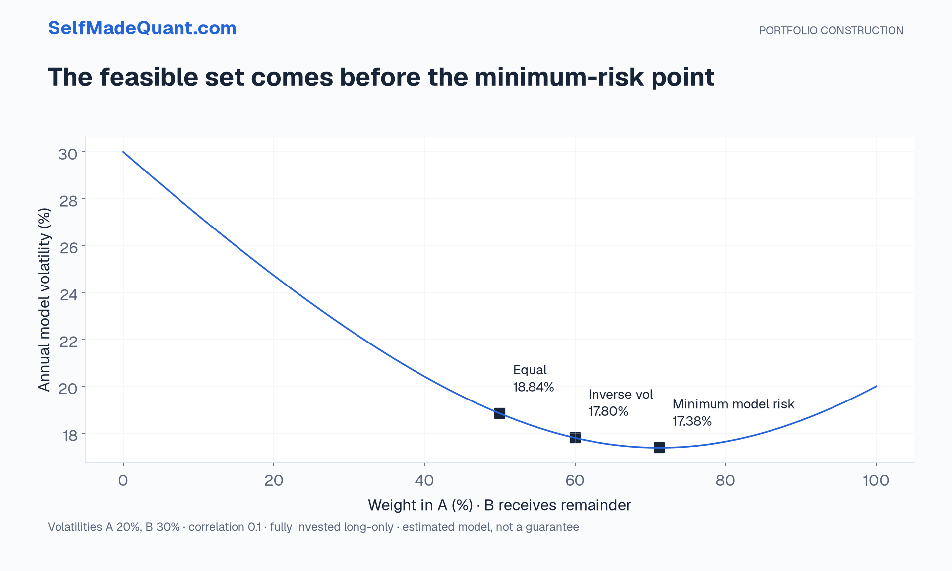
Equal weights give variance 0.0355. Inverse-volatility weights are 60/40 and give variance 0.03168. Differentiating the quadratic gives a minimum at weight 0.084/0.118, approximately 71.19% in A and 28.81% in B. Its volatility is about 17.27%.

These are results inside the supplied covariance model. The minimum-variance label does not mean lowest future realised risk among every possible strategy. Estimation error and changing joint behaviour remain outside this static calculation.

A risk contribution is not a capital weight

The marginal contribution to portfolio variance depends on how an asset covaries with the entire portfolio. Multiplying that marginal quantity by the asset weight gives a variance contribution; the contributions sum to total variance under the standard quadratic definition.

An asset with a small capital weight can still contribute substantial risk if it is volatile or loads strongly on the portfolio's common exposures. A hedging asset can have a negative contribution under some allocations. Decide whether you mean contribution to variance, volatility or a different risk measure before comparing numbers.

Inverse-volatility weighting equalises a particular capital-times-volatility expression. It does not generally equalise full portfolio risk contributions when correlations differ. The covariance structure is the missing part of that shortcut.

Holdings drift between trades

Suppose you start with equal weights and A rises 10% while B is unchanged. Before any rebalance, A's new weight is 0.55/1.05, approximately 52.38%. The portfolio did not remain at 50/50 merely because the target weights stayed unchanged.

A backtest that applies the same target weights every day implements daily rebalancing. A buy-and-hold experiment lets the weights drift. A periodic policy trades only at its stated boundaries. Those policies create different transactions and potentially different costs.

The target portfolio is a decision. Actual holdings are an account state. Keep both in the ledger so their differences are visible.

Make the proposed portfolio inspectable

Record the asset universe and labels, return horizon, covariance convention, objective, constraints, target weights and trading rule. Check the budget and exposure limits numerically after solving. Then inspect the trades required from the current holdings.

If the optimiser reports success, that confirms a computational stopping condition. It does not certify the quality of forecasts, the economic interpretation of constraints or the availability of the proposed trades.

Next we will keep the mandate fixed and change the estimated inputs. A small forecast adjustment can move weights much more than expected when the covariance model makes the relevant direction look almost riskless.

Until then, peace.