Financial time-series machine learning in Python: a reproducible experiment that fails out of sample

Published 14 October 2026Updated 15 October 20266 min readMachine learning for financial time series:Part 1 Part 2 Part 3Part 4

A useful financial machine-learning project should reproduce its data, timing rules, model-selection process and limitations. This Python experiment compares four admissible forecasts, exposes an impossible leakage control and records a final failure under a deliberately changed synthetic relationship.

The project uses NumPy and local files. It does not download market data, fit a live trading system or claim an investable return. Its small scope lets you audit the calculation before replacing the synthetic inputs with a harder dataset.

Read feature engineering and leakage, chronological model validation and baseline and cost comparisons for the reasoning behind each stage.

What does the Python project contain?

The package contains the source, 1,800 synthetic returns and signal values, a final prediction table, a JSON report and the illustrated explanations. The recorded seed is 20261014. The report stores the Python and NumPy versions used for the executed results.

Run python lab/time_series_ml_lab.py from the unpacked reader package with NumPy installed. The command regenerates synthetic_data.csv, final_predictions.csv and results.json. The article images are built from those saved outputs, rather than from manually chosen numbers.

Minor numerical differences can arise across numerical-library versions. The substantive checks concern information flow, accounting and reproducibility under the recorded environment; a fixed seed does not establish economic robustness.

Step 1: simulate a relationship with a declared break

The synthetic signal follows an autoregressive process. Return noise has a standard deviation of 1% per interval. Before session 1,200, the return's conditional mean has a positive coefficient on the previous signal. At session 1,200, that coefficient becomes negative.

y_t=\beta_t z_{t-1}+\epsilon_t,\qquad \beta_t=\begin{cases}0.003,&t<1200,\\-0.003,&t\ge1200.\end{cases}

The break is designed, disclosed and placed at the final boundary. It is not estimated from market history. We do not search alternative seeds or break dates for a more attractive story.

This creates a useful failure case: a real relationship in the earlier synthetic data need not remain useful after the generating rule changes. Removing the break would test a different, more stable process. Neither version can settle how much predictability exists in actual financial markets.

Frozen financial-ML models evaluated after a deliberately reversed synthetic relationship

Step 2: construct features available before execution

The decision is made before synthetic open t and the position earns the open-t to open-(t+1) return. The return immediately preceding that trade is not complete before open t, so it is excluded from features and from model-fitting labels at that boundary.

The feature row uses return y_(t−2), a five-return mean, a twenty-return standard deviation and a previous-close synthetic signal. The code requires a twenty-one-session warm-up. The signal's assumed publication time is part of the dataset contract.

Here is the core eligibility rule for a model fitted before a validation boundary:

import numpy as np

decisions = np.array([597, 598, 599, 600])
label_available_at_open = decisions + 1
eligible = label_available_at_open < 600
print(decisions[eligible].tolist())
# [597, 598]

Decision 599's label finishes at open 600. It is unavailable to a model fitted before that open. The example makes the strict inequality explicit instead of assuming that every preceding row is usable.

Step 3: declare the baselines and search

The admissible forecasting methods are zero return, the eligible training mean, ridge regression and a coarse shallow regression tree.

Ridge considers four penalties: 0, 0.1, 1 and 10 under the lab's mean-squared-loss normalisation. The tree considers four depth/minimum-leaf combinations: (1, 40), (2, 40), (3, 40) and (2, 100). At each node it evaluates nine quantile thresholds per feature.

These eight model configurations are the declared hyperparameter search. The fixed baselines are additional references. Feature design and the trading rule remain choices made by the researcher even though they are not counted as grid candidates.

Three expanding-window validation blocks select settings using mean squared return error. All fitted scaling comes from the corresponding training rows. After selection, the chosen models refit once on 1,178 eligible rows and remain frozen through 600 final decisions.

Validation selects ridge penalty 0.1 and tree depth three with minimum leaf forty. A production library may search splits differently from this teaching implementation. The source states exactly what this tree does.

Step 4: report the final loss and P&L separately

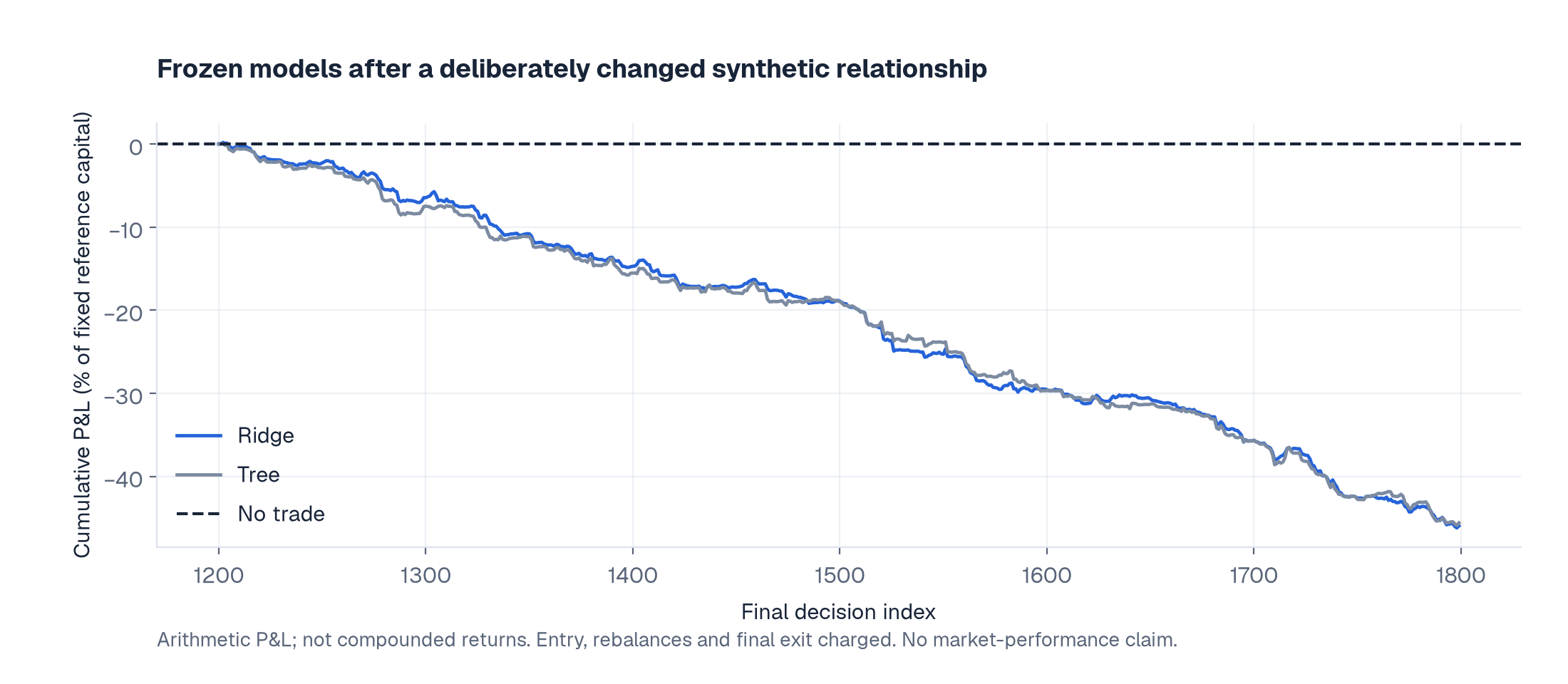
The final mean-squared errors are approximately 0.00010490 for zero, 0.00010479 for the training mean, 0.00012473 for ridge and 0.00012654 for the tree. Both ML models lose to the simple forecasts on this final metric.

The fixed position map clips predicted return divided by 1% to between −1 and +1. At five basis points per turnover unit, mean final net P&L is approximately −7.661 basis points per interval for ridge and −7.599 for the tree. The no-trade reference earns zero in the same accounting convention.

Entry, intermediate changes and final liquidation are charged. The cumulative P&L is measured on fixed reference capital. Borrow costs, nonlinear impact, financing, margin constraints and actual fill mechanics are not modelled.

The report also recalculates net P&L at zero, five and ten basis points per turnover unit without changing the fitted forecasts or position rule. That is cost sensitivity, rather than an opportunity to select the cheapest assumption after seeing the result.

Step 5: make leakage visibly impossible

The package intentionally includes one invalid control: using the target return as its own forecast. Its final MSE is exactly zero and its apparent trading P&L is spectacular. The report labels it leaked_target and keeps it outside the admissible comparison.

This is a positive control for a broken information boundary. It is not an estimate of how much leakage a real dataset contains. Its value is pedagogical: if your pipeline happily rewards future information, a high score alone cannot validate the experiment.

Two mutation checks then target specific causal boundaries. Replacing returns and signal values after session 900 leaves earlier feature rows unchanged. Changing future labels leaves predictions from an earlier fitted model unchanged.

The script also checks finite features, train-only scaling and turnover accounting. All six implemented checks pass. They do not certify publication timestamps, survivorship or execution feasibility for a dataset the project does not contain.

What would deployment monitoring add?

Monitor feature availability, freshness, missingness and distribution changes. Keep realised forecast errors and cost-adjusted trading results alongside those data-quality checks. Diagnose changes in inputs separately from changes in the feature–outcome relationship.

A drift alert is not an automatic instruction to retrain. Declare what triggers investigation, what data can enter a refit, how a replacement model is evaluated and when trading should pause. Otherwise the deployment process becomes another unrecorded model-selection loop.

Our final relationship reversal is known to the experiment's author. A deployed model would not know a real break date in advance. A monitoring policy needs a separate evaluation of detection delay, false alerts and the cost of its actions.

How should you extend this project?

Replace the generator with a point-in-time dataset and keep its publication history. Specify the tradable instrument and feasible order timing. Add relevant simple strategies, realistic costs and risk constraints. If labels have variable horizons, replace the fixed row exclusion with actual event-availability checks.

For a multi-asset dataset, split by the deployment question and preserve simultaneous information structure. For a new feature, log the hypothesis and available timestamp before inspecting its final performance. For a refitting policy, test the entire policy under the same label-eligibility rules.

What does this project demonstrate? A reproducible research process can identify that its selected models do not survive a designed distributional change. That is a useful result.

What does it not demonstrate? It does not establish that ML is ineffective in finance, that a particular model should be traded, or that a six-check script guarantees a leakage-free production system.

Download the code, data, outputs and twelve visual notes. Continue with the model decay and monitoring lesson.

References

Scikit-learn's leakage guidance and time-series split documentation provide implementation context. Bailey and co-authors discuss backtest selection risk. The data-generating process, numerical results and controls here are original synthetic teaching examples.

Until then, peace.