Machine learning for financial time series: build features without data leakage

Published 14 October 2026Updated 15 October 20265 min readMachine learning for financial time series:Part 1Part 2 Part 3 Part 4

Machine learning for financial time series means learning a relationship between information available at a decision time and an outcome observed later. The first task is to define those two times. A sophisticated estimator cannot repair a feature that contains the future.

A trading model can lose money even when its forecasts are genuinely out of sample. It can also look profitable because it was allowed to see information that did not exist when its trades supposedly happened. Those are different failures. This series keeps them separate through a small reproducible experiment.

We will define a forecast target, construct point-in-time features, choose models using chronological validation, translate predictions into positions, and inspect an intentionally difficult final sample. The Python data are synthetic. Their purpose is to make the information boundary visible, not to demonstrate a market anomaly.

What should a financial machine-learning model predict?

Start with the decision the prediction will support. A next-session return forecast, a probability of exceeding a loss threshold and a volatility forecast have different labels and evaluation criteria. “Predict the market” specifies none of them.

Our teaching target is the simple return from one synthetic session's opening price to the next opening price:

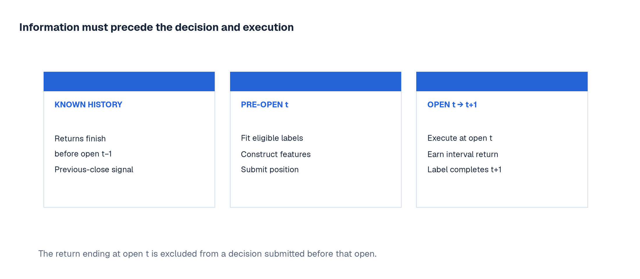
y_t=\frac{P^{\mathrm{open}}_{t+1}}{P^{\mathrm{open}}_t}-1.

The position is chosen before open t. The return y_t is not known until open t+1. A forecast made after observing open t cannot automatically claim execution at that same opening price. Real implementations need a feasible order-submission and execution convention.

The experiment therefore takes an explicit extra step back in return features: its most recent completed return is y_(t−2), which finished at open t−1. The immediately preceding return y_(t−1) finishes at open t and is excluded from the pre-open information set. A separate synthetic signal published at the previous close is available before open t.

This is a teaching convention with a conservative latency boundary. It does not model an actual exchange auction, opening spread or order queue. Those details would need to replace the synthetic execution assumption before using market data.

A forecast contract separates information availability, execution and label completion

What is data leakage in a trading model?

Data leakage occurs when model construction uses information unavailable under the experiment's stated decision-time rules. It can enter through the features, labels, fitted preprocessing, asset universe or model-selection process.

Suppose an earnings observation is labelled “quarter ending 31 March” but first published on 10 May. A strategy trading on 15 April cannot use that observation merely because a database keys it to March. The economically relevant fields include the period described, initial publication timestamp, later revisions and the version available to the researcher at the time.

A similar problem appears in sentiment data. A document timestamp may precede the vendor's processing time. A signal computed with a later model or corrected corpus may have a different availability history from the source document. Record which version the trading process could actually obtain.

Survivorship is another information error. Starting a historical equity study from today's surviving constituents can remove names that failed or left the universe. A clean train/test split does not restore the omitted securities. Universe membership must itself be point in time.

Price adjustments need provenance too. Corporate-action treatment should match the return you want to measure. A convenient adjusted series may be appropriate for one calculation while concealing the historical availability of information used in another feature. State the convention instead of treating every “adjusted close” column as interchangeable.

How do you construct causal financial features?

For this experiment, each feature row contains four values: the most recent eligible return, a five-return trailing mean, a twenty-return trailing standard deviation and a lagged synthetic signal. Every window ends before the decision boundary.

At decision index t, the return-based columns use slices ending at index t−2. In Python, the right endpoint of a slice is excluded:

def eligible_features(returns, signal, t):
    return [
        returns[t - 2],
        returns[t - 6:t - 1].mean(),
        returns[t - 21:t - 1].std(ddof=1),
        signal[t - 1],
    ]
# The twenty-return window requires a twenty-one-session warm-up.

The signal column has its own availability assumption: its t−1 value is known at the previous close. Lagging a column is useful only after understanding what its timestamp represents.

Rolling features should be explainable as a calculation someone could have performed then. A centered rolling average uses later observations. Backfilling a missing value from the future also crosses the boundary. A forward fill may be causally available but stale; add a freshness field or reject old observations when the economic meaning requires it.

Transformations fitted from data need the same discipline. Estimate a scaler, imputer, winsorisation threshold, feature selector or principal-component basis on training data, then apply it to the validation data. Refit these steps inside each validation fold. Scaling the complete dataset first lets future distributional information influence the training representation.

The scikit-learn leakage guide recommends splitting before fitted preprocessing and using pipelines to keep the operations together. A pipeline is useful machinery; it cannot infer whether a raw vendor field arrived after your proposed trade.

How can you test the information boundary?

One useful test changes data after a cutoff and recomputes earlier feature rows. Those earlier rows should remain identical. Our lab replaces future returns and future signal values after session 900; features for decisions before 900 do not change.

Another test alters labels after a training boundary and verifies that a model fitted strictly before that boundary gives identical predictions. These controls check particular information paths. They do not certify every feature source, execution assumption or historical revision rule.

Keep an explicit invalid control as well. The lab includes a “forecast” equal to the future target return. Its final mean-squared error is zero. That is a demonstration of an impossible information advantage, and it is excluded from the admissible model ranking. A spectacular score is sometimes evidence of a broken experiment.

Which baseline should you use before complex ML?

A return-prediction study should at least compare with a zero-return forecast and a mean estimated from eligible training returns. The corresponding trading decisions also need a no-trade baseline. A model can reduce forecast error without producing enough expected return to cover turnover costs.

These are deliberately weak-looking competitors. They make the incremental claim visible. If a model cannot beat a relevant simple forecast under the same clock, adding layers or trees changes the research question before it answers the first one.

This article's dataset is a single synthetic asset. Cross-sectional studies add simultaneous observations, shared events and asset identifiers. Splitting rows randomly can put the same date's economic shock on both sides. Decide whether the intended generalisation is to future dates, new assets or both, then group the evaluation accordingly.

Questions to settle before fitting

Does sorting by date eliminate leakage? No. A correctly sorted table can contain revised fundamentals, future-aware preprocessing or labels that were not yet complete.

Is a one-day lag always enough? No. Publication delays, label horizons and execution latency determine what is available. The experiment's one-session exclusion follows its stated pre-open convention.

Can feature selection use the final sample? If it does, that sample has influenced the research design. It can no longer serve as untouched final evidence for the revised feature set.

Next, time-series cross-validation for trading models turns these timing rules into train and validation boundaries. Review look-ahead bias in backtesting and the feature-engineering lesson for the surrounding research workflow.

Download the visual notes and runnable experiment.

References

Scikit-learn: common pitfalls and data leakage. The worked timing conventions and synthetic experiment are constructed for this series. No live trading results are claimed.

Until then, peace.