Market making with Python and public data: quotes, inventory, and what happens after a trade

Published 4 October 2026Updated 10 October 20269 min readMarket making:Part 1 Part 2Part 3

Suppose you quote both sides of a stock. Someone sells to your bid, so you buy below the current midpoint.

Have you made money?

That depends on what happens next. The price can fall after the trade, your inventory can accumulate, and costs can outweigh a small initial advantage.

In Part 1, we explored that problem with dice. In Part 2, we calculated conditional values, inventory risk, and a simple quote adjustment. This time, we will use real order-book data to measure the same ideas and build a small Python experiment.

The example has two steps. First, measure actual quotes and executions. Then try hypothetical quoting rules with a stated fill assumption. The first step describes historical data. The second depends on the assumptions we add to the simulation.

Start with data readers can download

We will use LOBSTER’s free AAPL, 21 June 2012, one-level sample. Get it from the provider’s sample-data page, or use this direct archive.

The archive provides a message CSV and an order-book CSV. The accompanying README explains their columns. These files contain historical Nasdaq data. They use the prices recorded in the sample, rather than today’s split-adjusted Apple prices.

Why use an order book instead of daily closing prices? We need to see the bid and ask separately, distinguish executions from other events, and preserve the sequence in which information arrives.

Download the accompanying Python script. It requires Python 3.10 or later, NumPy, and pandas. Install the two libraries with python -m pip install numpy pandas, then run python market_making_lab.py.

The script downloads the archive if the CSVs are not already available. Alternatively, unzip them into data/lobster/ yourself. You can select another folder with --data-dir.

It creates a local SQLite database, a table of execution measurements, and a table comparing quote experiments. No brokerage account or trading API is involved.

Understand the rows before calculating anything

These are the two input files:

AAPL_2012-06-21_34200000_57600000_message_1.csv
AAPL_2012-06-21_34200000_57600000_orderbook_1.csv

The message file contains time, event type, order ID, size, price, and direction. The book file contains the best ask price and size, followed by the best bid price and size.

One detail matters immediately: row

i

of the book is the state after message

i

. To compare an execution with the quote available before it, use the previous book row. Using row

i

to make a decision about event

i

would give the strategy information from after the event.

Another detail concerns direction. For a displayed execution, direction = 1 describes a resting buy order being executed. The participant with the resting order buys. The incoming seller sells to that order. A direction of -1 describes the passive sale. These conventions come from LOBSTER’s output specification.

The introductory loading calculation is:

from pathlib import Path
import numpy as np
import pandas as pd

folder = Path("data/lobster")
stem = "AAPL_2012-06-21_34200000_57600000"
messages = pd.read_csv(
    folder / f"{stem}_message_1.csv", header=None,
    names=["time", "event", "order_id", "size", "price", "direction"],
)
book = pd.read_csv(
    folder / f"{stem}_orderbook_1.csv", header=None,
    names=["ask", "ask_size", "bid", "bid_size"],
)
data = pd.concat([messages, book], axis=1)
data[["price", "bid", "ask"]] /= 10_000

print(len(data))
print(data.loc[0, ["bid", "ask"]].to_list())
# 118497
# [585.33, 585.94]

LOBSTER records dollar prices multiplied by 10,000. Dividing by 100 would produce the wrong scale. The complete script also checks row counts, chronological ordering, valid prices, and the absence of halt messages in this sample.

If working with files is new to you, start with SelfMadeQuant.com’s Reading and Writing Files lesson.

Measure the quoted market

The midpoint, spread, and displayed size imbalance are:

m_t=\frac{a_t+b_t}{2},\qquad s_t=a_t-b_t,\qquad I_t=\frac{Q_{b,t}-Q_{a,t}}{Q_{b,t}+Q_{a,t}}.

Here, $Q_b$ and $Q_a$ are the displayed quantities at the best bid and ask. The imbalance describes that displayed state. It does not tell us who will trade next.

data["mid"] = (data["bid"] + data["ask"]) / 2
data["spread"] = data["ask"] - data["bid"]
data["imbalance"] = (
    (data["bid_size"] - data["ask_size"])
    / (data["bid_size"] + data["ask_size"])
)

print(f"Median event-snapshot spread: ${data['spread'].median():.2f}")
# Median event-snapshot spread: $0.15

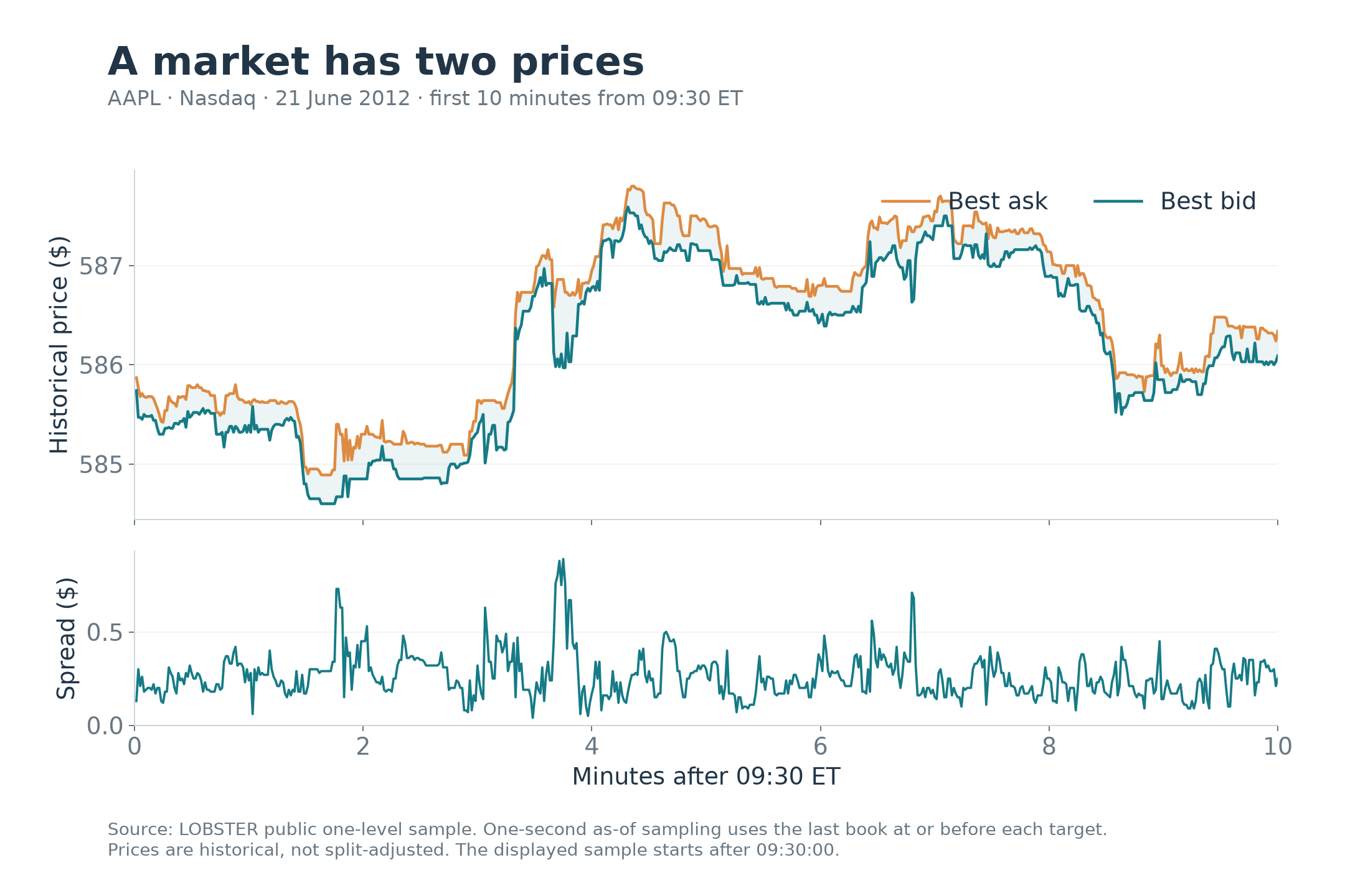
Each recorded event contributes one spread observation. Busy periods generate more events, so they contribute more observations to this median. A time-weighted statistic instead weights each quote by how long it remains in effect.

The first spread is $0.61, while the median across the sample is $0.15. A single opening snapshot is therefore a poor description of the entire day.

Historical AAPL best bid, best ask, and spread over the first ten minutes of the Nasdaq sample.

One-second as-of snapshots show the latest recorded book at or before each target time. The gap between bid and ask varies throughout these ten minutes; the historical prices are not split-adjusted.

What happens after an actual execution?

Take a displayed execution at price $p_t$ . Let $u_t=1$ for a passive purchase and $u_t=-1$ for a passive sale.

Its one-second markout, from the passive participant’s perspective, is:

\text{Markout}_{t,1s}=u_t(m_{t+1s}-p_t).

For a purchase, a later midpoint above the execution price gives a positive value. For a sale, a later midpoint below the execution price gives a positive value.

We can split the measurement into two pieces:

u_t(m_{t+1s}-p_t) =u_t(m_{t^-}-p_t)+u_t(m_{t+1s}-m_{t^-}).

The first term measures the execution price’s advantage relative to the midpoint before the event. The second measures the later midpoint move, with its sign adjusted for a purchase or sale.

The script selects event type 4, meaning a displayed execution, and excludes executions without a full remaining one-second horizon. At the target time, it uses the last recorded midpoint at or before that time. It does not use the next observation after the target.

Across the 23,646 eligible executions, weighting each measurement by executed shares gives:

Measurement	Dollars per share
Initial edge	+0.049562
Subsequent one-second movement	−0.046832
One-second markout	+0.002730

The accounting reconciles: $0.049562-0.046832=0.002730$ .

Waterfall showing initial edge of 0.049562 dollars per share reduced by subsequent movement of 0.046832, leaving a one-second markout of 0.002730.

Executed-share weighting across the 23,646 eligible displayed executions. The remaining markout is a midpoint valuation before fees, rather than a realised closing trade.

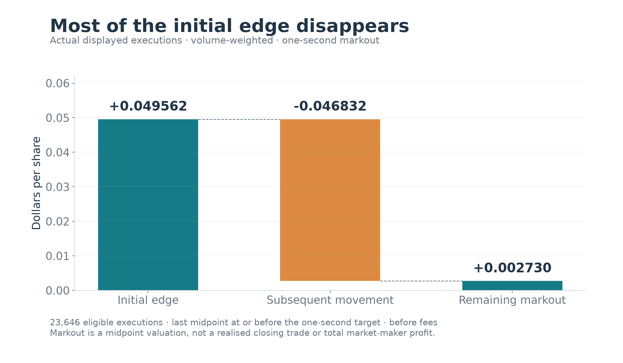
The later midpoint move removes most of the initial advantage in this historical sample. If we subtract an illustrative cost of $0.003 per share, the measured average becomes slightly negative. We assumed that cost for illustration. We do not know the actual fee paid by these participants.

A markout values a position at a later midpoint. It is not necessarily the price at which that position could be closed. It does not measure the market maker’s complete profit. The market maker may have hedged, held other positions, or traded at other venues.

For a deeper understanding of the average and the selection behind it, revisit Expectation, Mean, and Variance and Conditional Expectation.

Build a small database you can query

The complete script stores the data in market-making-output/market_making.sqlite with two tables:

Table	Contents
`book_events`	Original event sequence, prices, sizes, midpoint, spread, and imbalance
`passive_markouts`	Eligible displayed executions and their initial edge, subsequent move, and markout

The script stores a sequence number to preserve event order, even when several events have the same timestamp. Time alone is not a unique row identifier.

Once you have run the script, query the database:

import sqlite3

with sqlite3.connect("market-making-output/market_making.sqlite") as connection:
    result = connection.execute("""
        SELECT COUNT(*), ROUND(SUM(size * markout) / SUM(size), 6)
        FROM passive_markouts
    """).fetchone()

print(result)
# (23646, 0.00273)

This gives you a reproducible sample database built from the provider’s online files. You can now ask whether markouts differ by direction, spread, or displayed imbalance without repeatedly reading the original CSVs.

Such comparisons are descriptions of this day. Before testing on later data, fix the measurement horizon and grouping rules. Then check whether a feature that looked useful on this day remains useful.

Try a quote rule that responds to inventory

Now use the policy from Part 2:

c_t=m_t-\eta q_t,\qquad b_t=c_t-d,\qquad a_t=c_t+d.

We compare $\eta=0$ with $\eta=0.001$ dollars per share. Both start from a two-cent half-width, so the nominal full spread is four cents. The code rounds bids down and asks up to an assumed one-cent price grid. It then limits bids and asks so they do not cross the observed opposite quote.

For an isolated example with a $100 midpoint and 10 shares of inventory:

mid, inventory = 100.0, 10
skew, half_width = 0.001, 0.02
centre = mid - skew * inventory
bid = np.floor((centre - half_width) * 100 + 1e-8) / 100
ask = np.ceil((centre + half_width) * 100 - 1e-8) / 100

print(f"Bid: {bid:.2f}, ask: {ask:.2f}")
# Bid: 99.97, ask: 100.01

How do we decide whether a hypothetical order fills?

Suppose a displayed execution sells into a resting bid. If its price reaches or falls below our bid, we mark a candidate purchase. If an execution buys from a resting ask, its price must reach or exceed our ask to create a candidate sale.

We then use a seeded random draw with an assumed probability to choose a one-share fill. The code uses seed 42, an inventory limit of 100 shares in either direction, and the illustrative $0.003 fee per executed share. It makes decisions from the previous book row.

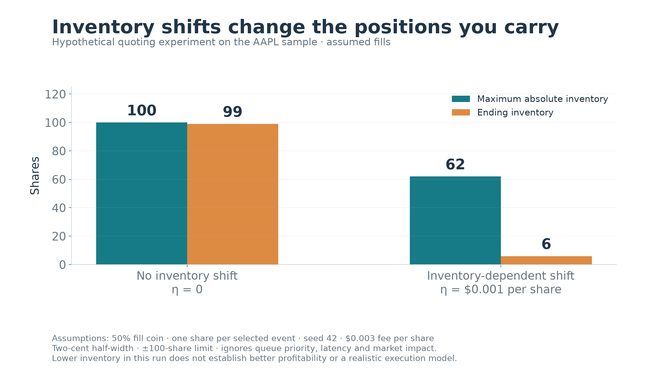
We vary the fill probability to see how results change. We have not estimated it from this dataset. Our four-cent quotes can offer better prices than the historical quotes. Adding those orders could therefore change how other participants trade. We also assume instantaneous quote updates and ignore queue priority, latency, hidden liquidity, and our own market impact. The experiment asks what these rules do under those assumptions.

At an assumed 50% fill probability, the script produces:

Result	No inventory shift	Inventory-dependent shift
Hypothetical one-share fills	9,415	8,898
Maximum absolute inventory	100	62
Ending inventory	99	6
Net terminal marked P&L	+$266.120	−$83.694

Hypothetical inventory comparison: maximum and ending inventory are 100 and 99 shares without a shift, versus 62 and 6 shares with an inventory-dependent shift.

This compares positions under the stated 50% fill assumption, one-share trades, seed 42, and illustrative fees. It illustrates inventory control in one run; the policy comparison does not establish superior profitability.

Terminal marked P&L is cash plus inventory valued at the final midpoint, after the assumed fees. It does not include an actual closing trade.

The inventory-dependent rule carries less inventory in this run. It also earns a lower marked profit. Reducing inventory risk does not guarantee higher realised profit on one price path.

The script also runs assumed fill probabilities of 25% and 100%. Both policies use the same seeded random draw for each event. Their quotes and inventories differ, so their candidate fills can differ too. Examine how the results change before drawing any conclusion about a policy.

The observed markouts earlier are measurements of real executions. The quote table is a hypothetical experiment. For a realistic strategy test, improve the execution model. Model when orders arrive and when cancellations take effect. Include suitable queue information and evaluate the strategy on later days.

What should you change next?

Start by changing the markout horizon from one second to five seconds. Does the initial edge still survive? Examine purchases and sales separately. Then group observations by spread or imbalance. Report the share count and event count for each group.

In the quote experiment, change the half-width, inventory shift, assumed fees, or fill probability one at a time. Explain how each change affects candidate trades and the positions you carry.

If you begin fitting a model, choose an earlier training period and evaluate on a later period. SelfMadeQuant.com’s Least Squares as Orthogonal Projection explains the fitting calculation; the timing and execution assumptions determine whether the fitted relationship is useful for the decision.

You can also practise the decisions without writing code in my free SelfMadeQuant.com Tools. The Market Making game lets you quote against noise traders and an insider; completing it requires a free account. The Order Book tool lets you examine how a market order consumes displayed liquidity. Together, they give the spread, information, inventory, and execution calculations a concrete setting.

By the end of this lab, explain each number in four steps. State what you observed, what you assumed, which position the trades created, and which price you used to value it.

Until then, peace.