What is statistical arbitrage? A pairs trade in six stages

Published 4 October 2026Updated 10 October 202610 min readStatistical arbitrage:Part 1Part 2 Part 3

You buy a stock because you think it is cheap. Then the whole market falls, and your stock falls with it.

Perhaps your valuation was sensible. Perhaps the company did better than its competitors. You can still lose money. Your position was exposed to the market’s direction as well as the company’s performance.

Now change the question. Instead of asking whether a stock will rise, ask whether it will outperform a related stock. Buy the relatively cheap one, sell the relatively expensive one, and study what happens to their relationship.

That is a useful starting point for statistical arbitrage: construct positions around a relationship estimated from data, then trade deviations that you expect to shrink.

Why do we expect the deviation to shrink? A historical relationship supports a hypothesis. It does not require future prices to return to that relationship.

Let’s build one trade from the beginning. We will use two fictional stocks, A and B. We will follow the cash through a winning trade, a losing trade, and a trade where both stocks rise.

This is Part 1 of a three-part series. Part 2 develops the maths, and Part 3 builds a small Python research project. Every price and trading result below is hypothetical.

Suppose A and B are businesses exposed to similar demand, input costs, and financing conditions. A broad change in their industry could move both stocks.

That gives us an economic reason to investigate a relationship. It does not establish that their prices should be equal. They may have different share counts, profit margins, debt, growth prospects, and exposure to the same industry shock.

“Same sector” helps us choose pairs to investigate. We still need to explain why a particular price relationship should persist.

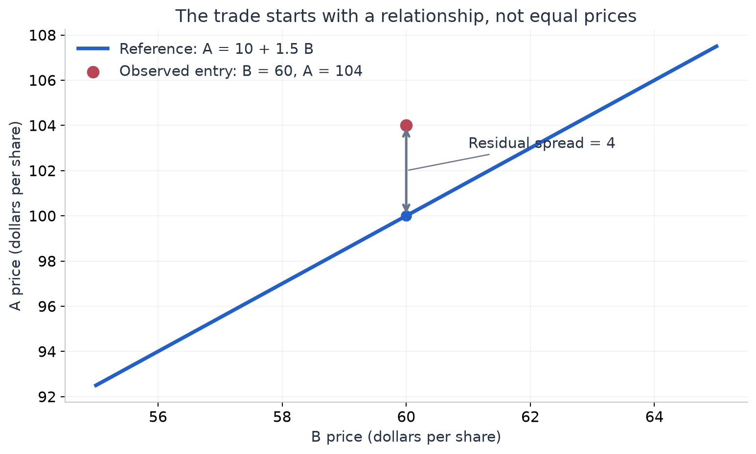
Imagine that a study of earlier observations suggests the following price-level model:

A_t=10+1.5B_t+s_t.

Both

A_t

and

B_t

are prices in dollars per share. The constant 10 and coefficient 1.5 are fixed for the examples in this article. The remaining term,

s_t

, is the residual spread:

s_t=A_t-10-1.5B_t.

At a B price of $60, the model’s reference price for A is:

10+1.5(60)=100.

If A trades at $104, the residual spread is 4. A is $4 above the model’s reference price.

Notice the qualification: above the model, rather than above a value we somehow know with certainty. The model could be stale or wrong.

We use regression to estimate relationships like this. Before trading, we also need evidence that the residual behaves in a useful way over time. A line can fit past observations closely while its residual keeps drifting on later observations.

A hypothetical price relationship and the four-dollar residual at entry

At B = 60, the model gives A = 100. The observed A = 104 sits four dollars above that reference. The line is an assumed relationship, not a valuation guarantee.

This also separates statistical arbitrage from textbook no-arbitrage arguments. A classical arbitrage constructs cash flows that cannot lose under its stated assumptions and can produce a gain. Our two companies have no contractual obligation to converge. We are forecasting a relative price move and accepting the risk that it does not occur.

Stage two: Turn the spread into a position

The residual is positive, so our hypothesis is that A is expensive relative to B. To benefit if the residual falls, we:

Short 100 shares of A at $104.
Buy 150 shares of B at $60.

Why 150 B shares? Because the price-level relationship puts a coefficient of 1.5 on B. For every 100 A shares we sell, we buy $100\times1.5=150$ B shares.

The hedge ratio is a share ratio in this example. If you estimate a coefficient from returns or log prices, translate it into trading quantities using those units. We cannot take any regression slope and automatically call it the number of shares to buy.

The opening cash flows are:

Opening transaction	Cash flow
Sell 100 borrowed A shares	+$10,400
Buy 150 B shares	−$9,000
Difference before costs	+$1,400

That $1,400 is not profit. We still owe 100 A shares and hold 150 B shares. We must eventually close both positions. The broker may also require collateral, which ties up capital.

A short sale means selling shares we do not own and later buying shares to return. The SEC’s short-selling explanation describes this borrowing and repayment mechanism for US equities. Actual availability, collateral, fees, and trading restrictions depend on the market and broker.

If A rises, buying it back becomes more expensive. The short position loses money. There is no fixed maximum loss from the short stock alone because its price has no fixed upper bound.

The long B position offsets some shared price movement. It does not remove all the short position’s risk. A can surge for company-specific reasons while B barely moves.

Also, we do not buy “10 dollars of intercept” for each share. The constant belongs to the reference relationship. With fixed coefficients, the intercept cancels when we calculate price changes. Cash and financing still belong in the trading account, but the intercept is not a third equity position.

Stage three: Follow a successful trade

Suppose we later observe:

A_T=102,\qquad B_T=61.

The new residual is:

s_T=102-10-1.5(61)=0.5.

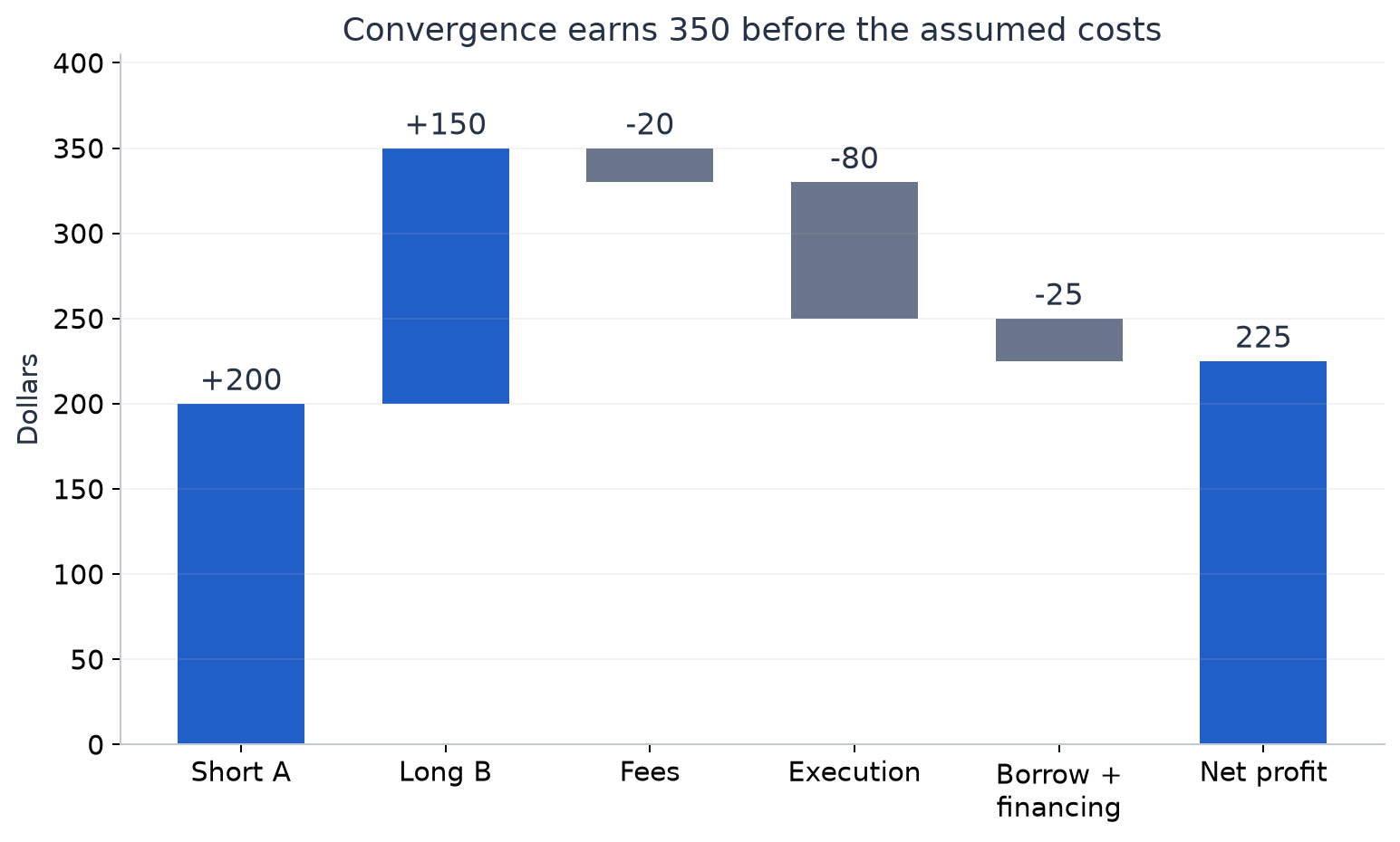
The residual has fallen from 4 to 0.5. We close the trade by buying back 100 A shares and selling the 150 B shares.

Leg	Calculation	Gross profit
Short A	$100(104-102)$	+$200
Long B	$150(61-60)$	+$150
Combined	$200+150$	+$350

There are two profitable legs here: the stock we sold fell, and the stock we bought rose.

But the more useful calculation is the portfolio calculation:

\begin{aligned} \Pi_{\mathrm{gross}} &=-100(A_T-A_0)+150(B_T-B_0)\\ &=-100(s_T-s_0)\\ &=100(4-0.5)=350. \end{aligned}

For this fixed-share, fixed-coefficient trade, the gross profit is proportional to the reduction in the residual spread. We did not need either price to return to its opening value.

Assume neither stock pays a dividend or other distribution during the hypothetical holding period. Now include an illustrative cost budget:

Cost over the entire trade	Amount
Commissions and exchange fees	$20
Bid–ask spreads and slippage	$80
Borrow and net financing	$25
Total	$125

The net profit is:

\Pi_{\mathrm{net}}=350-20-80-25=225.

These costs are assumed for the example, not typical market quotes. Holding the position longer can increase financing and borrow expense. Trading larger quantities can change execution costs.

If we forecast a smaller residual, the model gives us a possible gross profit. Subtract expected costs before deciding whether the trade is attractive.

Profit contributions from the two legs and the three assumed trading costs

The two legs make 350 dollars before costs. The assumed 125-dollar cost bill leaves 225 dollars. Opening short-sale proceeds are not included as profit.

Stage four: What if both stocks rise—or both fall?

A pairs trade does not require one stock to rise and the other to fall.

Keep the same opening position. Suppose B rises to $64 while A rises to $107. Both stocks are up, but the new residual is:

107-10-1.5(64)=1.

The short A leg loses $100(107-104)=300$ dollars. The long B leg makes $150(64-60)=600$ dollars. Combined gross profit is $300.

A rose by less than the model predicts for that increase in B. That relative change helped our position.

Now suppose B falls to $56 while A falls to $95. Again, the residual becomes 1:

95-10-1.5(56)=1.

The short A leg gains $900 and the long B leg loses $600. Gross profit is still $300.

Exit scenario	A price	B price	Exit residual	Gross profit
Both rise	107	64	1	+$300
Both fall	95	56	1	+$300
Original convergence example	102	61	0.5	+$350
A diverges upward	110	60	10	−$600

This is the attraction of relative-value trading: isolate a relationship more carefully than a simple outright purchase would.

Before calling the position “market neutral”, state which exposure the hedge removes.

At entry, we have $10,400 short and $9,000 long. The net stock dollar exposure is −$1,400. We are not dollar neutral. To equalise those dollar amounts we would buy about 173.33 B shares, but that would no longer match the model’s 1.5 share ratio.

A slope estimated from price levels is not automatically a market beta. Beta neutrality uses sensitivities to a chosen market factor and the dollar exposures of the positions. Even after we satisfy one hedge condition, sector, currency, volatility, and other exposures can remain.

A useful habit is to replace “neutral” with the exact statement: 100 A shares are hedged with 150 B shares according to this fitted price-level relationship. Then measure what risks remain.

Stage five: A relationship is not a rubber band

Why would we expect the residual to return?

Perhaps a lasting economic driver affects both companies. Temporary order flow or attention may then push their relative prices apart. That is a hypothesis we can investigate. Sometimes the apparent deviation is new information about one company, and the old relationship should change.

Correlation measures how two quantities vary together. Correlated daily returns can help identify shared risk, but they do not establish that a particular price-level spread remains bounded around a stable centre.

The related concept of cointegration concerns nonstationary series whose particular linear combination is stationary. Imagine two prices that share a wandering trend, with a residual that fluctuates around a stable level. The individual prices can travel far without the residual doing the same.

Granger’s Nobel lecture explains the common-trend idea behind cointegration. In trading, we still have to estimate the relationship and examine whether it survives on later data. A test result is evidence about a statistical model, not a promise about our next trade.

A synthetic mean-reverting residual followed by a permanent change in its centre

The second half shifts to a new centre. A rule anchored to the old mean could repeatedly sell a spread that has stopped being unusually high. This is an illustration, not market data.

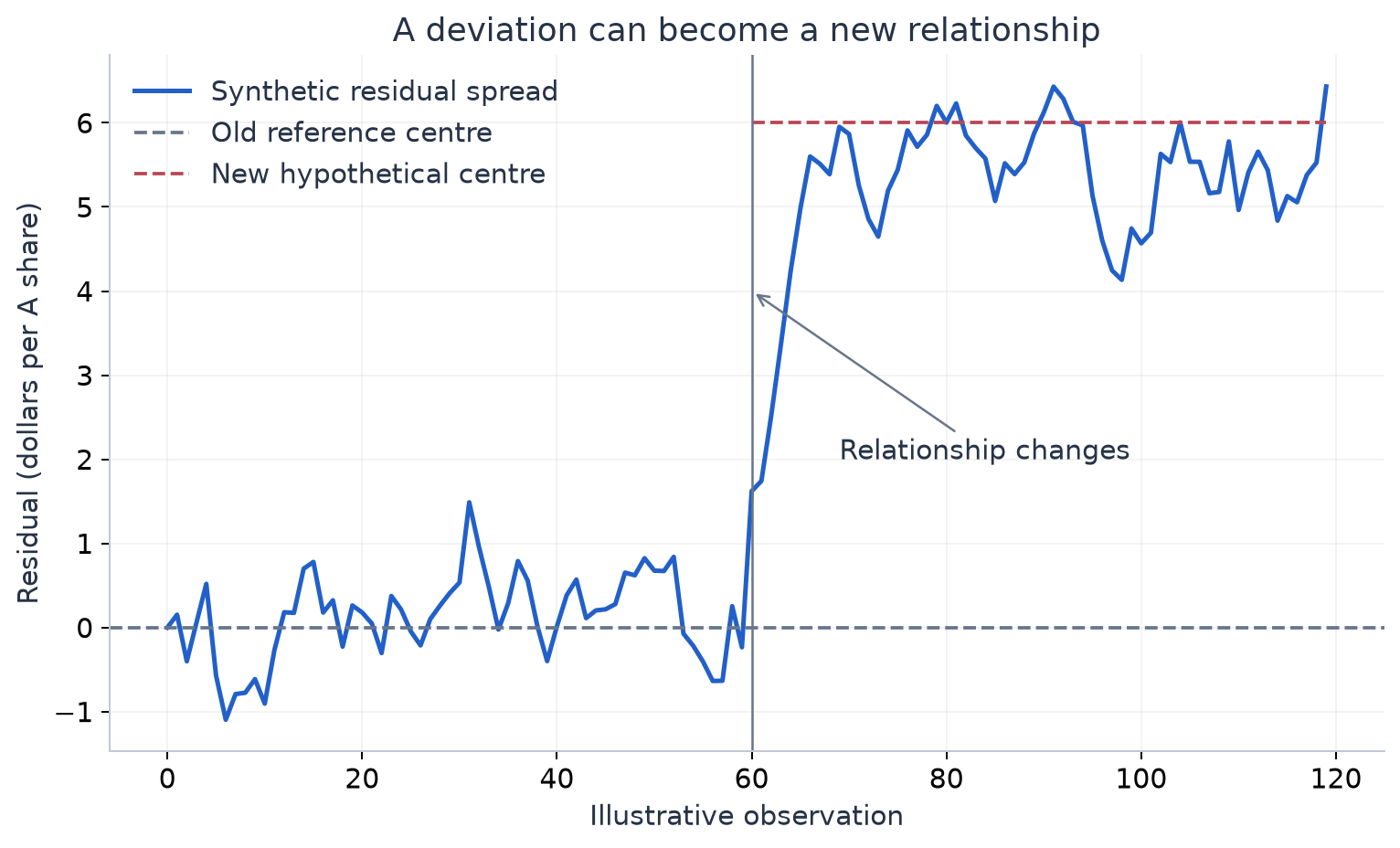
Return to our position. A rises to $110 while B stays at $60. The residual becomes 10, and gross profit is:

100(4-10)=-600.

The $600 loss exists before costs. The spread is now “even cheaper to short” according to the old model—but that interpretation is exactly what we must question.

A merger announcement, a change in business mix, deteriorating credit, or a persistent change in demand can alter a relationship. Borrow can also become unavailable or expensive before the prices converge.

Before trading, set a maximum holding period, exposure limits, and loss limits. Define when you will stop using the model. A stop triggers a planned response. It cannot guarantee the execution price, and it may close a position that later converges.

When prices disagree with the model, ask two questions. Does the deviation support a trading opportunity? Or does it show that the model needs to change?

Stage six: Decide whether the signal is worth trading

A residual of 4 is not meaningful without scale. If historical residual fluctuations are usually around 0.5, it may be unusual. If they are usually around 8, it may be ordinary.

A common summary is a standardised residual:

z_t=\frac{s_t-\mu_s}{\sigma_s}.

Here, $\mu_s$ and $\sigma_s$ are estimates from data available when the decision is made. If the estimated mean is 0 and standard deviation is 2, our entry residual of 4 gives $z=2$ .

The z-score measures distance from the estimated centre in units of estimated standard deviation. It is not automatically a probability of convergence, and “two standard deviations” is not automatically a profitable entry threshold.

Entry and exit rules need to connect that signal to a tradable account. Before opening our example trade, we would want answers to practical questions: Are both legs liquid? Can we borrow A? How quickly does the residual typically adjust? How large is the possible loss? Do expected costs consume the movement we hope to capture?

We also need an execution timeline. If the signal requires today’s completed close, calculate it after that close. Then state when you can submit orders and which prices you could trade. Do not assign the earlier closing price without explaining how execution there was possible. Realistic backtesting tests an implementable decision, including costs and financing, on observations not used to choose the rule.

The same idea extends beyond two stocks. We can hedge a stock with a basket, estimate residual returns after removing factor exposures, or allocate across many relative-value signals. More instruments can spread risk. But different positions may share factor exposures or attract the same traders. They can then lose money together.

The basic question remains: what relationship are we betting on, what position expresses it, and what evidence would tell us to stop?

Try the trade yourself

Keep the original position: short 100 A at $104 and long 150 B at $60. At exit, A is $101 and B is $59. The model coefficients remain fixed. Assume total costs are still $125.

What is the exit residual, the profit on each leg, and the net profit?

Worked answer. The exit residual is

101-10-1.5(59)=2.5

. The short A gains

100(104-101)=300

dollars. The long B loses

150(59-60)=-150

dollars. Gross profit is $150, which also equals

100(4-2.5)

. After $125 of costs, net profit is $25.

Both prices fell. One leg lost money. The spread still converged, and the portfolio made a small net profit. If actual costs exceeded $150, the same successful spread forecast would produce a losing trade.

Where this goes next

In Part 2, we turn the relationship into an estimated model, examine stationarity and mean reversion, and connect hedge weights to portfolio profit.

In Part 3, we build a reproducible Python project with data checks, a chronological research split, explicit position accounting, and trading costs. We will learn how to test a hypothesis. The data may show that no trade is worth taking.

For the underlying lessons, start with market neutrality and relative value, then study stationarity and tradable spreads, cointegration, and backtesting with costs and borrow.

References

US Securities and Exchange Commission, Key Points About Regulation SHO: short-sale borrowing and repayment mechanics in US equities.
Clive W. J. Granger, Time Series Analysis, Cointegration, and Applications, Nobel lecture, 2003: common trends and cointegration.