From spread to backtest: a statistical-arbitrage Python project

Published 4 October 2026Updated 18 October 20269 min readStatistical arbitrage:Part 1 Part 2Part 3

A spread can return to its average while your trade loses money.

You may enter after the move has already happened. You may change the hedge ratio while measuring the result. Or you may earn a small gross profit and spend more than that on execution and borrowing.

In Part 1, we built a pairs trade from two share prices. In Part 2, we examined the residual, its dynamics and the difference between statistical evidence and a trading forecast. Now we will build something readers can run: a small backtest with a cash ledger you can check.

The project has two exercises. A seeded synthetic pair lets us inspect every assumption and check the mechanics. A public historical IBM/SPY sample then tests whether a fitted relationship remains useful outside its formation window. The synthetic pair produces simulated trading results. The public sample produces historical price diagnostics. Keep those conclusions separate.

Download the project folder. It includes the scripts, two offline CSV fixtures, tests, result tables and three graphics. There is no brokerage account or live order submission.

Start with a controlled pair

We generate 500 business-date observations. B follows a random walk. A shares that movement but also carries a mean-reverting residual:

P_{B,t}=P_{B,t-1}+\epsilon_{B,t},\qquad P_{A,t}=10+1.5P_{B,t}+s_t,

s_t=0.88s_{t-1}+\epsilon_{s,t}.

The innovations are independent draws from seeded normal generators. This construction deliberately gives the pair a relationship. A profit in this simulation does not establish an edge in financial markets. It shows how the code behaves when the assumed relationship exists.

The script also generates opening prices separately from closes. The next opening price equals the previous close plus an independent overnight shock. A decision made after today's close can therefore execute at a different price tomorrow. This simple feature is enough to expose a common timing mistake.

Install the dependencies and run:

python -m pip install -r requirements.txt
python lab.py --charts
python -m unittest discover -v

NumPy and pandas handle the experiment. Matplotlib creates the optional charts. The default run writes its input to data/synthetic_pair.csv, so readers can inspect the observations or rerun without generating data:

python lab.py --csv data/synthetic_pair.csv

Every figure below describes synthetic observations. The business-date index excludes weekends but does not claim to reproduce a particular exchange's holiday calendar.

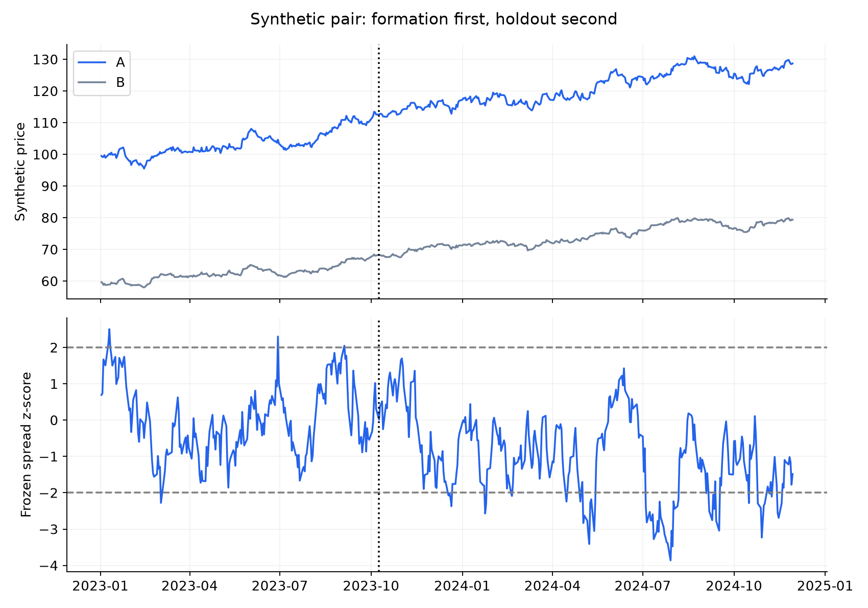
Synthetic prices and the frozen spread signal, with the formation boundary marked.

Fit once before measuring the holdout

The first 200 observations are the formation sample. The remaining 300 are the holdout. We estimate an intercept and a price-level hedge ratio using only formation closes:

(\widehat\alpha,\widehat\beta) =\underset{\alpha,\beta}{\operatorname{argmin}} \sum_{t=1}^{200}(P_{A,t}-\alpha-\beta P_{B,t})^2.

We also estimate the residual's sample standard deviation, then freeze all three quantities. The holdout signal is:

z_t=\frac{P_{A,t}-\widehat\alpha-\widehat\beta P_{B,t}} {\widehat\sigma_s}.

There is no separate residual mean subtraction here: OLS with an intercept makes the formation residual mean approximately zero. The denominator uses sample standard deviation, with ddof=1.

The fitted parameters from the actual run are:

from lab import synthetic, fit

prices = synthetic()
alpha, beta, scale = fit(prices)
print(f"alpha={alpha:.4f}, beta={beta:.4f}, scale={scale:.4f}")
# alpha=2.9353, beta=1.6055, scale=1.1151

The data-generating intercept was 10 and the slope was 1.5. A finite sample need not recover those exact values. Over this limited price range, different intercept and slope estimates can produce similar fitted prices. Treat the fitted numbers as estimates. State their units when using them.

For the underlying idea, revisit least squares. The fitted line makes a statement about the observations used to estimate it. The holdout is where we ask whether that statement remains useful.

Freezing the fit is a simple research design, not a claim that live strategies must never update. For a rolling design, specify the estimation window and refit dates. Record the share trades and cash flows required to update the hedge. We choose the fixed design because its signal and trading profit can be reconciled directly.

Write the trading rule before seeing the result

At each holdout close, a flat strategy checks whether $2\leq |z_t|<4$ . If the residual is positive, it targets short 100 A shares and long $100\widehat\beta$ B shares. If the residual is negative, it reverses both legs.

There is one position at a time. Its quantities stay fixed. We permit fractional B shares to preserve the price-hedge identity exactly. For broker execution, specify how you round quantities to permitted lots.

While holding, the strategy requests an exit if any of these occurs:

The residual reaches or crosses the mean-exit threshold: $z_t\leq0.5$ for a short spread, or $z_t\geq-0.5$ for a long spread.
The residual reaches $|z_t|\geq4$ .
The strategy has held the position through 20 closing observations.

Each request executes at the next observed open. The stop is therefore a decision threshold, not a promise to close at a particular price. An overnight gap can put the residual far beyond four standard deviations by the time the order executes.

The final exit is requested at the penultimate close and executed at the last open. We do not decide at the final close and pretend we could have traded that same closing price. Entries are disabled near the end so the experiment does not open a position with no planned trading horizon.

The rules are fixed for all three comparisons below. None was selected by searching for the highest reported profit. Avoiding that search makes the exercise easier to check. It does not make the synthetic process realistic.

Make signal time and execution time different columns

Suppose Monday's closing signal requests a short spread. The position remains flat overnight. It becomes short at Tuesday's open, and only then earns Tuesday's open-to-close movement.

If a position was already open, it gains or loses from Monday’s close to Tuesday’s open. That price change occurs before Tuesday’s order executes. The two intervals belong to different holdings:

\Pi_{t,\mathrm{gross}} =q_{t-1}^{\mathsf T}(O_t-C_{t-1}) +q_t^{\mathsf T}(C_t-O_t).

Here $O_t$ and $C_t$ are the two-asset opening and closing price vectors. The vector $q_{t-1}$ contains the old holdings. The vector $q_t$ contains the holdings after the opening trade.

This is why simply shifting a z-score and multiplying it by close-to-close returns can hide execution mistakes. That calculation may assign an overnight gain or loss to shares the strategy had not yet acquired.

The order CSV records both signal_date and execution_date. The ledger records actual shares and separates overnight and intraday contributions internally. A test raises the first entry's A opening price by one dollar. The new position pays the higher entry price. It cannot earn the price move that occurred before entry. The check verifies that the cash ledger responds correctly to a higher entry price.

Daily openings remain a simplified execution reference. We do not have simultaneous bid/ask quotes for the two legs, available depth or a guarantee of a fill at the recorded open.

Reconcile the shares, the residual and the cash

For a fixed short-spread holding $q=(-100,100\widehat\beta)$ , gross profit between two executable prices is:

\Pi_{\mathrm{gross}} =-100\Delta P_A+100\widehat\beta\Delta P_B =-100\Delta s.

The frozen intercept drops out of the change. It defines the residual's level but is not another security held in the account.

That identity fails if you compare residuals computed with different fitted parameters and call their change your fixed-share profit. Refitting can move a residual even when the traded prices do not change. Check the cash ledger. Buying shares reduces cash, and selling shares increases cash. At the close, add cash to the signed market value of all share positions to calculate equity.

At an opening trade, we charge:

K_t=\frac{b}{10000}\sum_j |\Delta q_{j,t}|O_{j,t}.

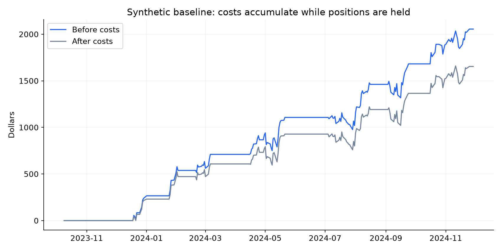
Baseline $b=5$ means five basis points of turnover on every leg, at entry and exit. We use this assumed charge to cover execution costs. It is not an observed spread or a broker’s fee schedule. The stress case uses 50 basis points.

Short borrowing costs three percent annually. We charge the marked short value for the actual calendar interval to the next observation, divided by 365. A Friday-to-Monday interval therefore costs three days. After the final exit, the account holds no short shares and incurs no further borrow charge.

We omit interest on cash, financing charges, collateral constraints, dividends, stock-lending recalls and margin calls. Those omissions are tolerable for a controlled mechanics exercise with synthetic no-dividend assets. They would materially affect a real equity strategy. Gross exposure can exceed the cash capital allocated to the strategy. Before expressing profit as an investment return, define the capital required.

Read the output before celebrating it

The verified run produced:

Synthetic case	Entries	Gross profit	Execution costs	Borrow costs	Net profit
Baseline	10	2,055.19	243.08	158.28	1,653.83
Cost stress	10	2,055.19	2,430.83	158.28	-533.92
Broken relationship	5	-305.99	117.40	63.00	-486.40

All monetary values are dollars for the stated share quantities. These are generated prices, not historical returns or a current opportunity.

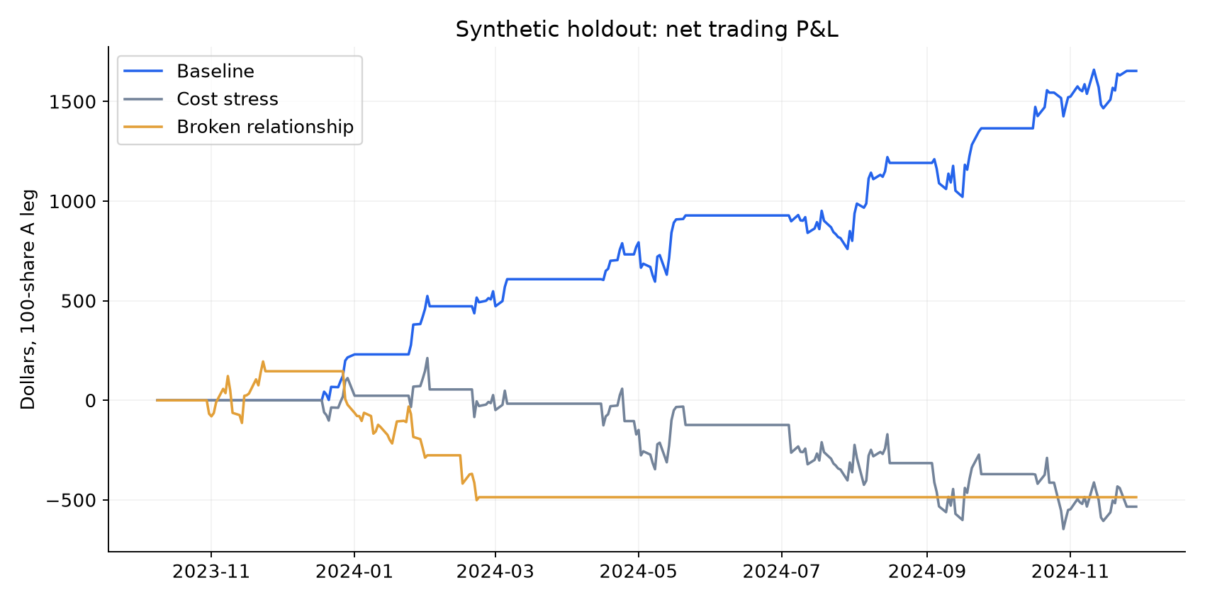
Synthetic baseline, cost stress and deliberately broken relationship: net P&L.

Increasing transaction costs leaves the signals and positions unchanged. Gross profit stays exactly the same. Net profit turns negative because the additional charge is nine times the baseline execution bill. Use this as an accounting check. If we change only the fee parameter, the strategy’s trading decisions should remain unchanged.

The broken-relationship case changes the holdout data, not the formation fit. A accumulates an extra 0.065 dollar drift per observation after the boundary. The old fitted relationship gradually stops describing the prices. Stop rules and the entry ceiling reduce the number of trades. They do not recover earlier losses.

The baseline maximum dollar drawdown is 199.45. It is the decline from a running P&L peak, including the initial zero. It is not a percentage drawdown on defined capital. Maximum gross exposure is 25,794.63 dollars, which helps explain why a 100-share instruction is not a full risk budget.

Synthetic baseline cumulative gross and net P&L.

Now inspect public prices without inventing a historical return

The package also includes 2020 daily IBM and SPY prices from the official QuantConnect/Lean sample repository. Readers can download these small sample files publicly. They do not require a commercial market-data subscription.

The source format is date/time, open, high, low, close and volume. Source prices are scaled integers, so the preparation divides them by 10,000. We retain dates, opening prices, and closing prices. Then we join the series on common dates. The package includes the resulting offline file, with its SHA-256 hash recorded in the README.

IBM versus SPY is a stock-versus-market diagnostic. It is not two interchangeable companies or a demonstrated cointegrated pair. We use it to ask a modest question: does a line fitted to the first part of 2020 continue to describe the later prices?

Run:

python public_data.py

The fixture has 253 matched observations. Formation uses the first 126; the remaining 127 are untouched holdout rows. Its frozen fit gives $\widehat\alpha=-8.2944$ , $\widehat\beta=0.4518$ and residual standard deviation 5.8191 dollars.

Holdout z-scores range from -6.3875 to -1.7704. Approximately 96.85% have absolute z-score at least two. This sustained departure challenges the assumption that the old fitted line remains a useful fair-value relationship. Repeatedly calling the deviation “cheap” would not solve the model's failure.

We intentionally report no historical trading profit. The fixture contains raw price bars, not a complete total-return or corporate-action ledger. Long dividends, short dividend obligations and appropriate action adjustments are needed before claiming equity strategy performance. Daily bars also do not establish simultaneous fills or stock-borrow availability.

This is a useful outcome for a research project: the data can reject the proposed relationship before we spend effort presenting a polished backtest.

Use the tests as questions about the economics

Five test methods pass in the delivered project. Together, they check that:

Changing future observations does not alter the fitted parameters or earlier ledger rows.
Every order executes after its signal.
Holdings follow the frozen share hedge, and the strategy closes all positions before the experiment ends.
Gross profit minus execution and borrowing costs equals final cash.
Increasing the cost parameter changes profit without changing positions.
A higher entry price increases the new position’s purchase cost. The position does not earn the earlier price gap.

The five test methods group these checks. They also check exits that cross beyond the exit band and rejection of invalid input. They do not prove profitability, stationarity or execution realism. They verify specific claims about the experiment’s timing, holdings, and cash accounting.

For a next project, introduce an explicit rolling formation scheme, realistic dividend cash flows and a capital allocation rule. Keep a later period untouched while choosing those rules. Then compare several pairs with economic reasons for their relationships. Record each rejected pair as well as any successful pair.

The deliverable is an inspectable experiment: data, a forecast, delayed decisions, holdings, cash flows and a holdout. A smooth spread chart is only the beginning.