The maths of statistical arbitrage: from a fitted spread to a trade

Published 4 October 2026Updated 10 October 20269 min readStatistical arbitrage:Part 1Part 2Part 3

A pair of stocks can move together for years and still lose money when you trade the gap between them. A regression can fit past prices closely while its residual keeps drifting. A spread can mean revert while its expected profit is smaller than the cost of entering and exiting.

The mathematics helps us separate those questions.

In Part 1, we used an invented price relationship:

A_t=10+1.5B_t+s_t.

Here $A_t$ and $B_t$ are prices in dollars per share at time $t$ . The residual $s_t$ is the difference between A's observed price and its model estimate. It is measured in dollars per A share. The intercept 10 is also in dollars per A share. The slope 1.5 converts a dollar move per B share into a predicted dollar move per A share.

When A was $104 and B was $60, the model estimate for A was $100. The residual was $4. We sold 100 shares of A and bought 150 shares of B.

But where did 10 and 1.5 come from? Why should $4 be unusual? And what evidence would make us expect it to fall?

Estimate the relationship before judging the gap

Suppose these five artificial observations are our training sample. We use a small sample so you can calculate the fit by hand. Five observations do not establish a trading strategy.

Observation	B price	A price	Fitted A price	Residual
1	$58.00	$98.00	$97.00	$1.00
2	$59.00	$97.50	$98.50	−$1.00
3	$60.00	$100.00	$100.00	$0.00
4	$61.00	$100.50	$101.50	−$1.00
5	$62.00	$104.00	$103.00	$1.00

Ordinary least squares chooses an intercept

\hat\alpha

and slope

\hat\beta

to minimise the sum of squared residuals:

\min_{\alpha,\beta}\sum_{t=1}^{n}(A_t-\alpha-\beta B_t)^2.

For one explanatory variable and an intercept, the solution is:

\hat\beta= \frac{\sum_t(B_t-\bar B)(A_t-\bar A)} {\sum_t(B_t-\bar B)^2}, \qquad \hat\alpha=\bar A-\hat\beta\bar B.

The bars denote sample averages. In our table, $\bar B=60$ and $\bar A=100$ . Subtract each series’ average to centre its values. The centred B values are $-2,-1,0,1,2$ . The centred A values are $-2,-2.5,0,0.5,4$ .

The numerator is:

(-2)(-2)+(-1)(-2.5)+(0)(0)+(1)(0.5)+(2)(4)=15.

The denominator is $4+1+0+1+4=10$ . Therefore:

\hat\beta=15/10=1.5, \qquad \hat\alpha=100-1.5(60)=10.

Five invented observations, the fitted line A equals 10 plus 1.5 B, and vertical residuals.

The vertical gap measures the residual. The fitted line describes how these prices vary together at the same time. It does not predict how the next residual will behave.

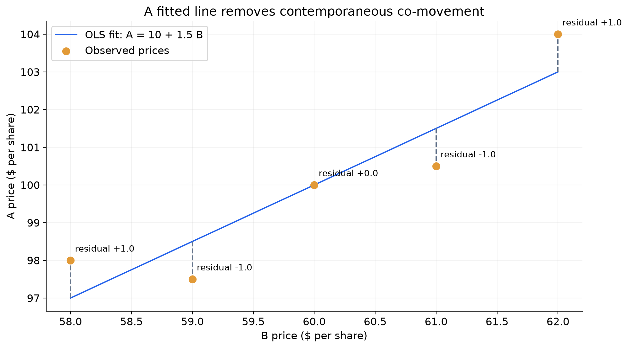
Our residuals sum to zero. Their centred cross-product with B is also zero:

\sum_t\hat s_t=0, \qquad \sum_t(B_t-\bar B)\hat s_t=0.

These are algebraic consequences of this least-squares fit with an intercept. Regression geometry describes them as orthogonality to the fitted explanatory directions.

They are not evidence that the residual is stationary, independent, normally distributed, or likely to reverse tomorrow. The fit makes the historical errors satisfy these equations. It does not establish a future equilibrium.

Checkpoint. Using the fitted model, what is the residual when A is $104 and B is $60? It is

104-10-1.5(60)=4

. The observation is a deviation from a historical relationship, not a theorem that A must fall to $100.

Correlation asks a different question from cointegration

Return correlation describes whether percentage changes tend to move together. Cointegration concerns whether a particular combination of nonstationary price levels has a stationary residual.

A simple counterexample makes the distinction visible. Suppose:

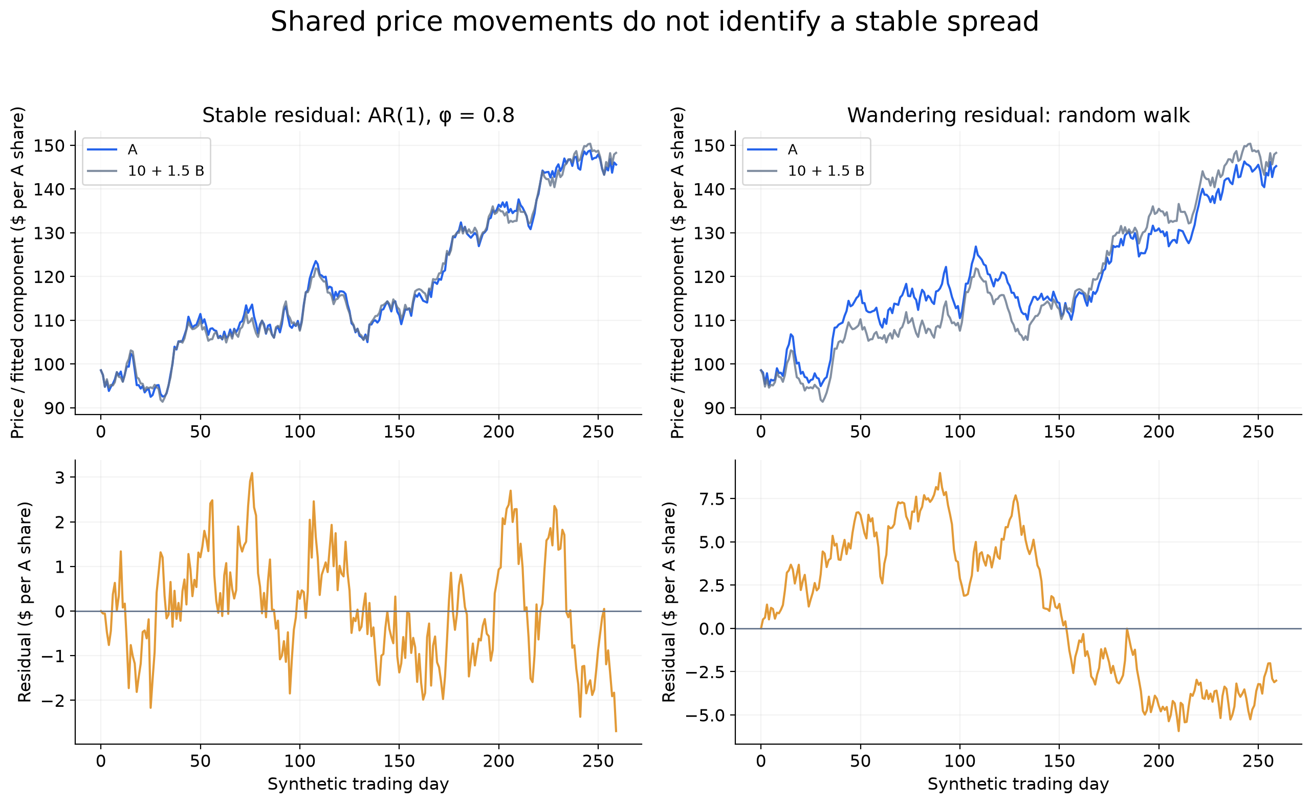
\begin{aligned} B_t&=B_{t-1}+u_t,\\ A_t&=A_{t-1}+1.5u_t+v_t, \end{aligned}

where $u_t$ is a common random shock and $v_t$ is an independent additional shock. Both have zero mean and finite variance. If the common shock dominates, the two price changes will be highly correlated. When price changes are small relative to price levels, their percentage returns can also look strongly related.

Yet the spread satisfies:

s_t=A_t-1.5B_t-10=s_{t-1}+v_t.

It is a random walk. Its conditional expected next value is its current value, and its variance grows with time. Similar daily movements have not created a restoring force.

Compare that with a model in which the residual itself follows:

s_t=0.8s_{t-1}+\varepsilon_t.

Assume independent shocks with zero mean and constant finite variance. If we also start the residual in its stationary distribution, this residual is stationary. If B is a random walk and A equals $10+1.5B+s$ , the two prices can share a nonstationary trend while their specified combination remains stationary.

Synthetic prices with a common component and either a stationary AR(1) residual or a wandering random-walk residual.

Both constructions share a price driver. Only the left construction imposes a stable residual. These are teaching simulations, not empirical test results.

Stationarity gives a statistical framework for a stable distribution through time. Real companies can change their business mix, capital structure, or exposure to commodity prices. A relationship can cease to hold even after a convincing historical test.

Test the fitted residual using the right reference distribution

First check whether each candidate price series plausibly has a unit root, so it is integrated of order one, or I(1). The Engle–Granger approach then fits the price relationship and tests the estimated residual for a unit root. The null is no cointegration.

One residual-test regression has the form:

\Delta\hat s_t =\gamma\hat s_{t-1} +\sum_{j=1}^{p}c_j\Delta\hat s_{t-j}+e_t.

Here $\Delta\hat s_t=\hat s_t-\hat s_{t-1}$ , $p$ is the number of lagged changes, $c_j$ are coefficients, and $e_t$ is the regression error. The lagged changes help account for dependence between observations over time. Under the unit-root null, $\gamma=0$ ; a sufficiently negative test statistic can support rejection.

The important implementation detail is that

\hat s_t

was estimated from the same observations. Its test statistic needs cointegration-specific critical values. Do not report an ordinary ADF p-value on the fitted residual as an Engle–Granger result. That p-value uses the wrong reference distribution.

For a formal Engle–Granger test, statsmodels.tsa.stattools.coint implements the appropriate reference distribution. Its documentation specifies the I(1) assumption, first-stage deterministic terms, and MacKinnon-based p-values and critical values. An intercept-only relationship and a relationship with a deterministic time trend represent different hypotheses. Source: statsmodels cointegration test documentation.

An illustrative decision would be: if a test statistic were $-3.6$ and the returned 5% critical value were $-3.4$ , reject at that level because $-3.6<-3.4$ . These numbers are hypothetical. Use the actual critical values returned for your specification and sample.

Rejection does not identify an entry threshold or establish profitability. Failure to reject does not prove the absence of a relationship. Testing hundreds of pairs also creates a selection problem. Account for that search when judging the smallest p-value. It is not equivalent to one test chosen in advance. Preserve a separate period for evaluating the selected strategy.

Convert the residual into an unusualness score

A $4 residual may be enormous for one pair and routine for another. Standardisation puts the gap on the scale of its historical fluctuations:

z_t=\frac{s_t-\hat\mu}{\hat\sigma}.

Here $\hat\mu$ is an estimated residual mean and $\hat\sigma$ is an estimated residual standard deviation, both in dollars per A share. Their ratio is dimensionless.

Suppose a separate training window with substantially more observations gives $\hat\mu=0$ and $\hat\sigma=2$ . Our $4 residual gives $z=2$ . A residual of $0.50 gives $z=0.25$ .

A rule might enter a short-spread position above 2 and exit when the score falls below 0.5. These are candidate rules to evaluate, not universal trading constants.

A score of 2 is not automatically a 97.5th-percentile event. That interpretation requires a suitable distributional model. Financial residuals may have skew, heavy tails, serial dependence, and changing volatility.

For a clean first experiment, estimate the mean, standard deviation, and hedge coefficients on training data and freeze them during evaluation. If you instead update them, specify exactly which past observations were available at each decision. A larger estimated standard deviation can reduce the z-score even if prices have not converged profitably. Updating the intercept can move the model’s reference level toward a losing position. That model change does not recover the loss.

Estimate the speed of adjustment

A stationary residual can revert too slowly to trade economically. While you wait, you pay borrow and financing charges and keep capital committed to the position.

A simple autoregressive model is:

s_{t+1}=a+\phi s_t+\varepsilon_{t+1}.

The intercept $a$ has residual-dollar units. The persistence $\phi$ is dimensionless. Assume independent, zero-mean innovations of fixed finite variance. If $|\phi|<1$ , the stationary mean is $\mu=a/(1-\phi)$ .

Writing $x_t=s_t-\mu$ gives $x_{t+1}=\phi x_t+\varepsilon_{t+1}$ . Repeated conditional expectations imply:

\mathbb E[x_{t+h}\mid x_t]=\phi^h x_t.

For $0<\phi<1$ , the half-life of this expected deviation is:

h_{1/2}=\frac{\log(1/2)}{\log\phi}.

With daily observations and $\phi=0.8$ , this is about 3.11 trading days. A $4 deviation has conditional expected deviations of $3.20 after one day, $2.56 after two, and $2.048 after three.

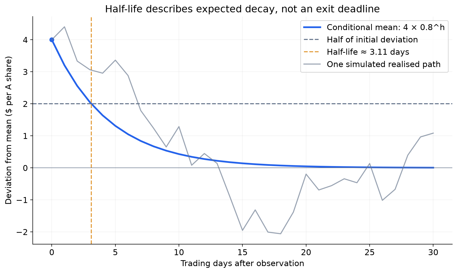
Expected decay from a four-dollar residual, its 3.11-day half-life, and one noisy simulated path.

The smooth curve describes a conditional mean. An individual path can rise, cross the mean early, or remain away from it much longer.

Check the boundary cases before interpreting a half-life. As $\phi$ approaches 1 from below, the half-life grows without bound. At $\phi=1$ , there is no finite restoring half-life. Values with $|\phi|>1$ are explosive in this causal model. At $\phi=0$ , the expected deviation disappears at the next observation. For negative $\phi$ with magnitude below one, the conditional expected deviation alternates in sign. You can use $|\phi|$ to calculate how quickly its amplitude halves. The expected path no longer moves steadily toward the mean. At $\phi=-1$ , shocks also prevent stationary finite-variance behaviour under these assumptions.

A continuous-time Ornstein–Uhlenbeck model writes the restoring force as $dx_t=-\kappa x_t\,dt+\eta\,dW_t$ . Here $\kappa>0$ is a rate in inverse time, $\eta$ is residual volatility per square root of time, and $W_t$ is Brownian motion. Its exact sampled persistence is $\phi=e^{-\kappa\Delta t}$ , giving half-life $\log2/\kappa$ . This is a useful next model. The daily AR(1) already answers our immediate question: how quickly does the fitted conditional mean decay?

Estimated persistence is uncertain, especially near one or in short samples. A point estimate of three days is not a guaranteed holding period or an automatic stop-loss rule.

Return to our trade: short 100 A and long 150 B. Keep those quantities fixed until exit.

If A falls from $104 to $102 while B rises from $60 to $61, the gross profit is:

\begin{aligned} \Pi&=-100(102-104)+150(61-60)\\ &=200+150=350. \end{aligned}

The residual fell from 4 to $102-10-1.5(61)=0.5$ . Since our coefficients stayed fixed:

\Pi=-100\big[(A_1-A_0)-1.5(B_1-B_0)\big] =100(s_0-s_1)=350.

Subtract $125 of assumed total execution, borrow, and financing costs, and the net result is $225. The intercept cancels from the price change. It is not a $1,000 cash payment earned when we enter.

This identity explains why the slope matters for sizing. Shorting 100 A and buying 100 B would leave an additional exposure to B's movement. The residual chart would no longer measure the price changes of the portfolio we actually hold.

If we change the hedge coefficient while holding a position, spread changes also contain model changes:

\Delta s_t=\Delta A_t-\beta_{t-1}\Delta B_t -B_t\Delta\beta_t-\Delta\alpha_t.

The last two terms change the chart even when they produce no trading profit. Actual portfolio profit uses the quantities held over each interval. Track cash when rebalancing. Buying more shares uses cash. Changing the short position changes both cash proceeds and the shares you owe. Record each trade and its cost. Do not treat a residual change caused by refitting as trading profit.

Choose the neutrality you actually intend

At entry, our A short has value $10,400 and our B long has value $9,000. Net risky-asset dollar exposure is −$1,400. The price-regression hedge is therefore not dollar neutral.

To be dollar neutral at those prices, 100 short A shares would require $10{,}400/60\approx173.33$ long B shares. That is a different portfolio from the 150-share statistical hedge.

Market-beta neutrality is different again. If the return betas to a market factor are $b_A$ and $b_B$ , approximate dollar market-factor exposure is:

q_AA_tb_A+q_BB_tb_B,

where signed quantities $q_A,q_B$ are positive for longs and negative for shorts. Setting this to zero need not match either dollar neutrality or the price-regression ratio. Sector, currency, and commodity exposures can also survive the hedge.

A log-price regression creates another distinction:

\log A_t=\alpha+\beta\log B_t+s_t.

For small moves,

\Delta s\approx\Delta A/A-\beta\Delta B/B

. Thus

\beta

acts locally as a dollar-exposure ratio. A corresponding small-move share hedge uses

q_B=-q_A\beta A/B

; it does not use

q_B=-q_A\beta

as the price-level model does. This is a local approximation, not an exact fixed-share P&L identity for log-spread changes.

Before coding, write down whether your model uses prices or logs, what its slope means, and which risk you want the positions to offset.

Turn the equations into a reproducible experiment

The steps now connect. Fit a relationship using past data and examine its residual. Estimate the deviation’s size and adjustment speed. Translate the signal into share quantities. Then calculate profit and costs from the actual trades.

In Part 3, we build a small Python project around that sequence. The main output is a trade ledger you can check: data known at the signal time, actual entry and exit quantities, holding period, gross profit, and deductions.

For the underlying mathematics, continue with linear regression, stationarity and unit roots, and cointegration and error correction.

The test can support a relationship. The ledger tells us whether our chosen implementation earned money under its stated assumptions.